Properties of the Normal Distribution
Many real-world measurements, like height and weight, usually cluster around an Average Value, with fewer cases at the extreme high or low ends. This pattern forms a bell-shaped curve known as the normal distribution.
A normal distribution is fully determined by two key values: the mean (\(\mu\)) and the standard deviation (\(\sigma\)). Because it is symmetric and unimodal, the mean, median, and mode are always equal. The spread of the data depends on \(\sigma\) — when \(\sigma\) is small, the values are closely packed around the mean, forming a narrow bell curve. Conversely, a larger \( \sigma \) means the data is more spread out, creating a wider, more dispersed bell shape.
Z-Scores
The \(Z\)-Score measures how many Standard Deviations a Data Point (\( x \)) is away from the Mean (\( \mu \)). A positive Z-Score indicates the value is above the Mean, while a negative Z-Score indicates the value is below the Mean.
Characteristics of the Z-Score:
- A \(Z\)-Score of 0 means the data value is exactly equal to the mean (\(\mu\))
- Positive \(Z\)-Scores indicate values greater than the mean (\(\mu\))
- Negative Z-Scores indicate values less than the mean (\(\mu\))
- The \(Z\)-Score converts a Normal Distribution to the Standard Normal Distribution, which has a mean of 0 and a Standard Deviation of 1
Using the \(Z\)-Score, we can find the Probability of a value occurring within a Normal Distribution by referring to the Areas Under the Curve of the Standard Normal Distribution.
The \(Z\)-Score can be expressed algebraically as such:
Where:
- \(x\) is the Value from the Data Set
- \(\mu\) is the Mean of the Data Set
- \(\sigma\) is the Standard Deviation of the Data Set
The Difference Between Exponential and Normal Distribution
The Exponential Distribution is asymmetric, meaning it has a Peak at zero and a long tail on one side. This means events are most likely to happen quickly (i.e. a short wait), and the chance of longer waits decreases. It’s used for situations like waiting times or time between random events.
The normal distribution, or bell curve, is symmetric, meaning both sides of the curve are the same. Most values are close to the middle (mean), and fewer values are found at the extremes. It’s often used to model things like people’s heights, where most are near average and fewer are very short or tall.
Example
Alex is 165cm tall. The heights of women in his city are normally distributed with a mean of 160cm and a standard deviation of 8cm. What is the probability that a randomly selected woman from his city will be taller than Alex?
First, we can identify the given information:
- Alex's height: \(x = 165 \; [\text{cm}]\)
- Mean height of women: \(\mu = 160 \; [\text{cm}]\)
- Standard Deviation: \(\sigma = 8 \; [\text{cm}]\)
Next, we can calculate the \(Z\)-Score using its corresponding formula:
\(z = \cfrac{x - \mu}{\sigma}\)
\(z = \cfrac{165 - 160}{8}\)
\(z = \cfrac{5}{8}\)
\(z = 0.625\)

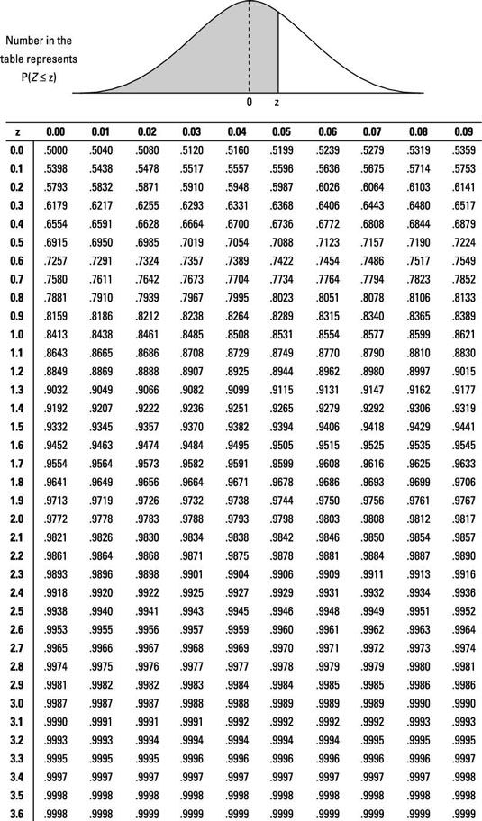
Using the \(Z\)-Score table above, a \(Z\)-Score of 0.625 corresponds to a Cumulative Probability that lies between 0.7234 and 0.7357. Averaging these two values gives us the following result:
This gives a Cumulative Probability of approximately 0.734, meaning the Probability that a woman will be shorter than Alex is 0.734.
To find the Probability that a woman will be taller than Alex, subtract this Cumulative Probability from 1:
\(P(\text{taller than Alex}) = 1 - P(\text{shorter than Alex})\)
\(P(\text{taller than Alex}) = 1 - 0.734\)
\(P(\text{taller than Alex}) = 0.266\)
Therefore, we can determine the probability that a woman will be taller than Alex is approximately 0.266.
A group of 120 students participated in a science quiz. The Average Score was 72% with a Standard Deviation of 6%. Determine the Percentile Rank of each of the following students:
- Emily, who scored 85%
- Ryan, who scored 62%
- Sophia, who scored 95%
First, we can identify the following information:
- Mean Score: \(\mu = 72\%\)
- Standard Deviation: \(\sigma = 6\%\)
- Number of students: \(120\)
Next, we can calculate the \(Z\)-Score for each student using the following formula:
- Emily, who scored 85%:
Ryan, who scored 62%:
Sophia, who scored 95%:
Using the \(Z\)-Score table from the earlier example, a \(Z\)-Score of 2.17 corresponds to a Cumulative Probability of approximately 0.9850, meaning Emily’s Percentile Rank is 98.50%.
Using the \(Z\)-Score table from the earlier example, a \(Z\)-Score of -1.67 corresponds to a Cumulative Probability of approximately 0.0475, meaning Ryan’s Percentile Rank is 4.75%.
Using the \(Z\)-Score table from the earlier example, a \(Z\)-Score of 3.83 corresponds to a Cumulative Probability of approximately 0.9999 (since it’s extremely high and close to 1), meaning Sophia’s Percentile Rank is 99.99%.
Therefore, we can summarize the final answers as such:
- Emily’s Percentile Rank is 98.50%
- Ryan’s Percentile Rank is 4.75%
- Sophia’s Percentile Rank is 99.99%
The weights of apples in a grocery store are Normally Distributed with a Mean of 150 grams and a Standard Deviation of 20 grams. What is the Probability that an apple weighs between 130 grams and 180 grams?
First, we can identify the following information:
- Mean Weight: \(\mu = 150 \; [\text{g}]\)
- Standard Deviation: \(\sigma = 20 \; [\text{g}]\)
- Range: \( x_1 = 130 \; [\text{g}]\) to \( x_2 = 180 \; [\text{g}]\)
Next, we can calculate the \(Z\)-Scores for the bounds using the formula:
For \(x_1 = 130 \; [\text{g}]\):
For \(x_2 = 180 \; [\text{g}]\):
A \(Z\)-Score of -1.00 corresponds to a Cumulative Probability of 0.1587.
A \(Z\)-Score of 1.50 corresponds to a Cumulative Probability of 0.9332.
Calculate the Probability between these \(Z\)-Scores:
\(P(130 < x < 180) = P(z_2) - P(z_1) = 0.9332 - 0.1587 = 0.7745\)
\(P(130 < x < 180) = 0.9332 - 0.1587 = 0.7745\)
\(P(130 < x < 180) = 0.7745\)
Therefore, the Probability that an apple weighs between 130 grams and 180 grams is approximately 0.7745 or 77.45%.