Normal Sampling and Modelling

Normal sampling and modelling involves selecting a small but representative group (or sample) from a larger population to draw conclusions about the whole. This is especially useful when measuring the entire population isn’t practical.

If the population follows a normal distribution - where most values are concentrated around the average, forming a bell-shaped curve — the sample will typically reflect that pattern. By analyzing the sample, we can make reliable predictions about the entire population. The larger the sample, the more accurately it represents the population, improving the reliability of our conclusions.

Although normal distributions often involve continuous data, they can also be used to model discrete data, such as the number of earthquakes that you count in whole numbers. Even though it’s not continuous like height or time, if you have a large enough set of this data and it forms a symmetric, bell-shaped pattern with one peak, a statistician might fit a smooth normal curve to it. Once that curve fits, they can use it to make predictions about the data, just like they would with continuous data.

Formulas

Z-Score

The \(Z\)-Score formula calculates how far a value is from the mean in standard deviations:

\(z = \cfrac{x - \mu}{\sigma}\)

Where:

\(z\) is the \(Z\)-score (standardized value)
\(x\) is the observed value (i.e. height)
\(\mu\) is the population mean
\(\sigma\) is the population standard deviation

Standard Error

The Standard Error measures the variability of the sample mean:

\(SE = \cfrac{\sigma}{\sqrt{n}}\)

Where:

\(SE\) is the standard error
\(\sigma\) is the population standard deviation
\(n\) is the sample size

Example

A researcher measures the heights of 50 randomly selected adults and finds the average height is 170cm with a standard deviation of 10cm. Assuming the population is normally distributed, what’s the probability that a randomly chosen person from the population is taller than 180cm?

First, we can identify the following information:

Mean Height: \(\mu = 170 \; [\text{cm}]\)
Standard Deviation: \(\sigma = 10 \; [\text{cm}]\)
Observed Value: \(x = 180 \; [\text{cm}]\)
Sample Size: \(50\) (not directly used here, but confirms population normality assumption)

Next, we can calculate the \(Z\)-Score as such:

\(z = \cfrac{x - \mu}{\sigma}\)

\(z = \cfrac{180 - 170}{10}\)

\(z = \cfrac{10}{10} = 1\)

A \(Z\)-Score of 1 means 180cm is 1 standard deviation above the mean.

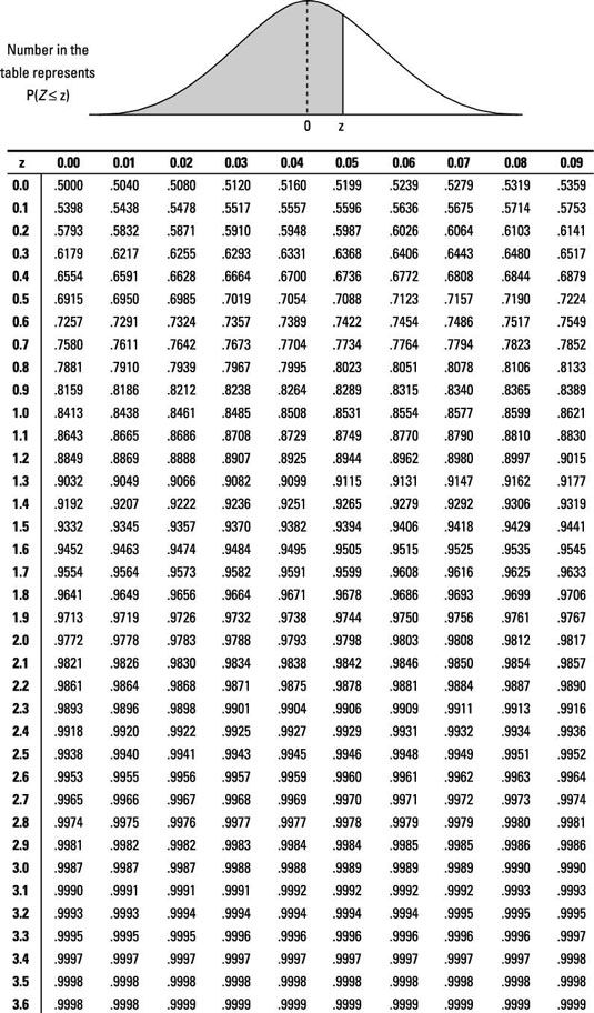
Using a standard normal table above, the probability of being less than \(z = 1\) is approximately 0.8413, or 84.13%.

Since we want the probability of being greater than 180cm, we can subtract 0.841 from 1:

\(P(x > 180) = 1 - 0.8413\)

\(P(x > 180) = 0.1587\)

Therefore, the probability that a randomly chosen person is taller than 180cm is approximately 0.1587 or 15.87%.

A company tests the battery life of 100 phones and gets an average of 20 hours with a standard deviation of 2 hours. If they use a normal model, how would the spread of the sample means change if they tested 400 phones instead?

Show Answer

First, we can identify the following information:

Mean Battery Life: \(\mu = 20 \; [\text{hours}]\)
Standard Deviation: \(\sigma = 2 \; [\text{hours}]\)
Initial Sample Size: \(n_1 = 100 \)
New Sample Size: \(n_2 = 400 \)

Next, we can calculate the Standard Error, \(SE\), using the following formula:

\(SE = \cfrac{\sigma}{\sqrt{n}} \)

For 100 phones:

\(SE_1 = \cfrac{2}{\sqrt{100}} = \cfrac{2}{10} = 0.2 \text{ hours}\)

For 400 phones:

\(SE_2 = \cfrac{2}{\sqrt{400}} = \cfrac{2}{20} = 0.1 \text{ hours}\)

The spread of the sample means is the Standard Error, which decreases from \(0.2 \; [\text{hours}]\) to \(0.1 \; [\text{hours}]\).

This means that the spread gets halved because a larger sample size reduces the standard error, thereby making the sample mean more precise.

Therefore, we can determine the spread of the sample means would decrease from 0.2 hours to 0.1 hours.

A city records the number of daily car accidents over 200 days, with an average of 5 accidents per day and a standard deviation of 2. Since the data is discrete but forms a bell shape, how could a statistician use a normal model to predict the chance of having 8 or more accidents in a day?

Show Answer

First, we can identify the following information:

Mean Accidents: \(\mu = 5/[\text{day}]\)
Standard Deviation: \(\sigma = 2 \)
Observed Value: \(x = 8 \; [\text{accidents}]\)
Sample Size: \(200 \; [\text{days}]\) (supports normal approximation)

Since the data is discrete but bell-shaped with a large sample, we can approximate it with a normal model as stated earlier.

Next, we can calculate the \(Z\)-Score for \(8\) accidents as such:

\(z = \cfrac{x - \mu}{\sigma} \)

\(z = \frac{8 - 5}{2}\)

\(z = \frac{3}{2} = 1.5\)

A Z-Score of \(1.5\) means \(8\) accidents is \(1.5\) Standard Deviations above the mean.

Using the Standard Normal table from above, the probability of being less than \( z = 1.5 \) is approximately \(0.9332\) (or \(93.32\)%).

For 8 or more accidents, we want the area above 1.5. In order to find the percentage of this occuring, we can subtract \(0.9332\) from \(1\):

\(P(x \geq 8) = 1 - 0.9332 = 0.0668\)

\(P(x \geq 8) = 0.0668 \)

Therefore, a statistician would use the normal model to estimate about a 6.68% chance of \(8\) or more accidents in a day.