Rational Functions with Linear Terms
Rational Functions with Linear Terms represent polynomial functions in which both the numerator and denominator are linear expressions. They can be expressed algebraically as:
- \(a\) helps shift the Horizontal Asymptote
- \(b\) represents the Vertical Stretch/Compression
- \(c\) represents a Horizontal Stretch/Compression. It also helps shift the Horizontal Asymptote
- \(d\) shifts the Vertical Asymptote
A rational function can also be represented algebraically in the form:
As with base reciprocal functions, the denominator (in this case \(q(x)\)) cannot equal \(0\). Otherwise, this would make the entire function undefined.
Additionally, both the numerator and denominator are only allowed to contain variables with degrees of 1.
Since there is a variable in both the numerator and denominator, there are effects on both the vertical and horizontal asymptotes and consequently, the domain and range.
Characteristics of Rational Linear Functions
Domain
The Domain of rational functions with linear terms is all real numbers where \(x\) cannot equal the Vertical Asymptote, \(\{x\in\mathbb{R}, x \ne d\}\).
Range
The Range of rational functions with linear terms is all real numbers where \(x\) cannot equal the Horizontal Asymptote, \(\{y\in\mathbb{R}, y \ne a/c\}\).
Asymptotes
Vertical Asymptotes are vertical lines that a function cannot cross, thereby restricting its domain. For a rational function with linear terms, the VA can be determined by setting the denominator equal to \(0\) and solving for \(x\), provided the numerator doesn’t have the same \(0\). Otherwise, these terms will cancel out.
Horizontal Asymptotes are horizontal lines that a function approaches as its inputs, \(x\), approaches or \(-\infty\). Unlike its vertical counterpart, a Horizontal Asymptote can be crossed. For a rational function with linear terms, the HA can be determined by dividing each term in both the numerator and denominator by \(x\) and investigating the behavior of the function as \(x \rightarrow \pm \infty\).
Additionally, it should be noted that both branches are equidistant from the point of intersection of the vertical and horizontal asymptotes.
Intercepts
The \(y\)-intercept can be determined by substituting \(0\) for \(x\) and solving for \(f(x)\).
The \(x\)-intercept can be determined by setting the numerator equal to \(0\) and solving for \(x\).
Example
Determine the intercepts, domain, range, asymptotes, and end behaviours of \(s(x) = \cfrac{2x + 6}{3x -9}\). Then, sketch a graph of the function.
First, we can determine its intercepts. We can determine its \(y\)-intercept by substituting \(0\) for \(x\):
\(s(0) = \cfrac{6}{-9}\)
\(s(0) = -\cfrac{2}{3}\)
Next, we can determine its \(x\)-intercept by setting the numerator equal to \(0\) and solving for \(x\):
\(0 = 2x + 6\)
\(2x = -6\)
\(x = -3\)
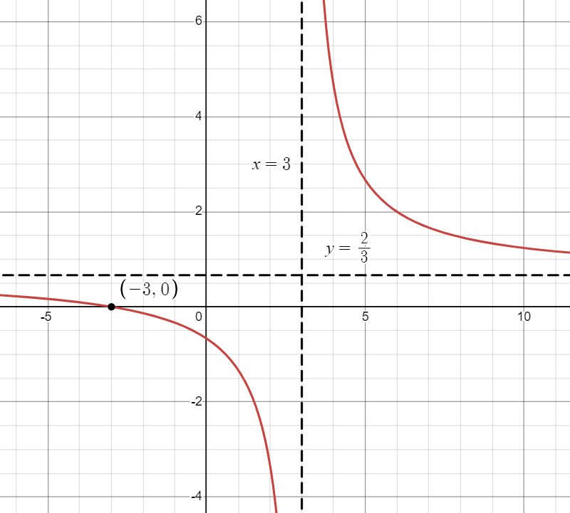
Therefore, we can determine that the \(y\) and \(x\)-intercepts are \(\boldsymbol{\left(0, -\cfrac{2}{3}\right)}\) and \(\boldsymbol{(-3,0)}\) respectively.
Then, we can determine the function’s asymptotes. We can start with its Vertical Asymptote by setting the denominator equal to \(0\) and solving for \(x\):
\(\text{VA}: 0 = 3x - 9\)
\(\text{VA}: 3x = 9\)
\(\text{VA}: x = 3\)
Next, we can determine the function’s Horizontal Asymptote by dividing both sides by \(x\) and determining its end behaviors:
\(\text{HA}: y =\cfrac{2}{3}\)
After, we can determine the function’s domain. Since we have determined that the function contains a vertical asymptote at \(\boldsymbol{x=3}\), we can identify that the domain is restricted at this point. As a result, we can express the domain as \(\boldsymbol{\{x\in\mathbb{R} |x \ne 3\}}\).
We can also determine that function’s range. Since we have determined that the function contains a horizontal asymptote at \(\boldsymbol{y = 2/3}\), we can identify that the range is restricted at this point. As a result, we can express the range as \(\boldsymbol{\left\{y\in\mathbb{R} |y \ne \cfrac{2}{3}\right\}}\).
Finally, we can determine the function’s end behaviors:
| As \(\boldsymbol{x \rightarrow}\) | \(\boldsymbol{s(x) \rightarrow}\) |
| \(- \infty\) | \(2/3\) |
| \(3^-\) | \(-\infty\) |
| \(3^+\) | \(+\infty\) |
| \(+ \infty\) | \(2/3\) |
Using the information we have determined above, we can draw a sketch of the function as such:
First, we can determine its intercepts. We can determine its \(y\)-intercept by substituting \(0\) for \(x\):
\(t(0) = \cfrac{-2}{-1}\) \(t(0) = 2\)
Next, we can determine its \(x\)-intercept by setting the numerator equal to \(0\) and solving for \(x\):
\(0 = -5x - 4\)
\(5x = -2\)
\(x = -0.4\)
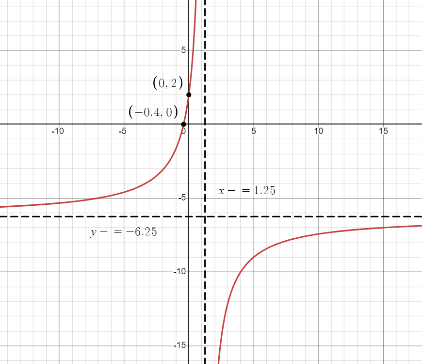
Therefore, we can determine that the \(y\) and \(x\)-intercepts are \(\boldsymbol{(0, 2)}\) and \(\boldsymbol{(-0.4,0)}\) respectively.
Then, we can determine the function’s asymptotes. We can start with its Vertical Asymptote by setting the denominator equal to \(0\) and solving for \(x\):
\(\text{VA}: 0 = 0.8x - 1\)
\(\text{VA}: 0.8x = 1\)
\(\text{VA}: x = 1.25\)
Next, we can determine the function’s Horizontal Asymptote by dividing both sides by \(x\) and determining its end behaviors:
\(\text{HA}: y = -6.25\)
After, we can determine the function’s domain. Since we have determined that the function contains a vertical asymptote at \(\boldsymbol{x=1.25}\), we can identify that the domain is restricted at this point. As a result, we can express the domain as \(\boldsymbol{\{x\in\mathbb{R} | x \ne 1.25\}}\).
We can also determine that function’s range. Since we have determined that the function contains a horizontal asymptote at \(\boldsymbol{y= -6.25}\), we can identify that the range is restricted at this point. As a result, we can express the range as \(\boldsymbol{\{y\in\mathbb{R} |y \ne -6.25\}}\).
Finally, we can determine the function’s end behaviors:
| As \(\boldsymbol{x \rightarrow}\) | \(\boldsymbol{t(x) \rightarrow}\) |
| \(- \infty\) | \(-6.25\) |
| \(1.25^-\) | \(+\infty\) |
| \(1.25^+\) | \(-\infty\) |
| \(+ \infty\) | \(-6.25\) |
Using the information we have determined above, we can draw a sketch of the function as such: