Reciprocal Linear Functions
A Reciprocal Linear Function occurs when a polynomial is divided by a linear expression. This function is expressed algebraically as:
- \(k\) represents the slope
- \(c\) represents the horizontal shift or Vertical Asymptote
- \(d\) represents the vertical shift or Horizontal Asymptote
Characteristics of Reciprocal Linear Functions
Domain
The domain of reciprocal linear functions is all real numbers where \(x\) cannot equal \(c\) over \(k\), \(\{x\in\mathbb{R}, 𝑥 \ne c/k\}\). You can evaluate reciprocal linear functions for almost any real \(x\)-value.
The restriction on the domain of a reciprocal linear function can be determined by finding the value of \(𝑥\) that makes the denominator \(0\). This value can be expressed as:
Range
The range of reciprocal linear functions is all real numbers except for \(d\), \(\{y\in\mathbb{R} | y > d\}\).
As \(d\) represents the number of units the function is vertically translated, it also represents the Horizontal Asymptote, and by extension, the restriction on the range.
Asymptotes
Vertical Asymptotes are vertical lines that a function cannot cross, thereby restricting its domain. The Vertical Asymptote for a Reciprocal Linear Function can be determined by using the following equation:
Horizontal Asymptotes are horizontal lines that a function approaches as its inputs, \(x\), approaches or \(−\infty\). Unlike its vertical counterpart, a Horizontal Asymptote can be crossed. The Horizontal Asymptote for a reciprocal linear function is represented by \(d\). If there is no \(d\) value, the default HA is \(𝑦=0\).
Slope
The Slope of a reciprocal linear function depends on its \(k\) value, assuming that \(𝑦=0\).
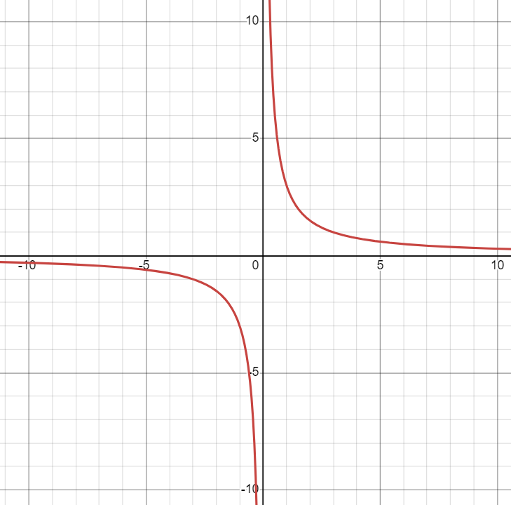
If \(k>0\), the left branch has a negative, decreasing slope, and the right branch has a negative, increasing slope:
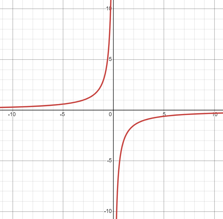
If \(k< 0\), the left branch has a positive, increasing slope, and the right branch has a positive, decreasing slope:
Intercepts
The \(y\)-intercept can be determined by substituting \(0\) for \(x\) and solving for \(f(x)\). A reciprocal linear function can have only 1 \(y\)-intercept.
The \(x\)-intercept(s) can be determined by setting the numerator equal to \(0\) and solving for \(x\). If the function doesn’t have a \(d\)-value, then the function won’t have any \(x\)-intercepts. If the function has a \(d\)-value, then the function will have one \(x\)-intercept.
End Behaviours
The end behavior for the respective branches of reciprocal linear functions are dependent on the \(k\)-value and are summarized in the table below assuming the HA is \(𝑦=0\):
| \(k\)-value | Left Branch | Right Branch |
|---|---|---|
| Positive | \(x \rightarrow -\infty, y\rightarrow 0\) \(x \rightarrow \cfrac{c^-}{k}, y\rightarrow -\infty\) |
\(x \rightarrow \cfrac{c^-}{k}, y\rightarrow +\infty\) \(x \rightarrow +\infty, y\rightarrow 0\) |
| Negative | \(x \rightarrow -\infty, y\rightarrow 0\) \(x \rightarrow \cfrac{c^-}{k}, y\rightarrow +\infty\) |
\(x \rightarrow \cfrac{c^-}{k}, y\rightarrow -\infty\) \(x \rightarrow +\infty, y\rightarrow 0\) |
Graphing
In order to graph a reciprocal linear function, it’s good to know a few of its key characteristics first in order to sketch it more accurately. These include:
- Domain. Determine restrictions by identifying the Vertical Asymptote
- Range. Determine restrictions by identifying the Horizontal Asymptote
- Behavior Around Vertical Asymptote. Does each branch approach infinity or negative infinity around this Asymptote?
- End Behaviors. Does each branch lie above or below the Horizontal Asymptote when x approaches positive or negative infinity?
- Intercepts. Do they exist? Where are they located?
Example
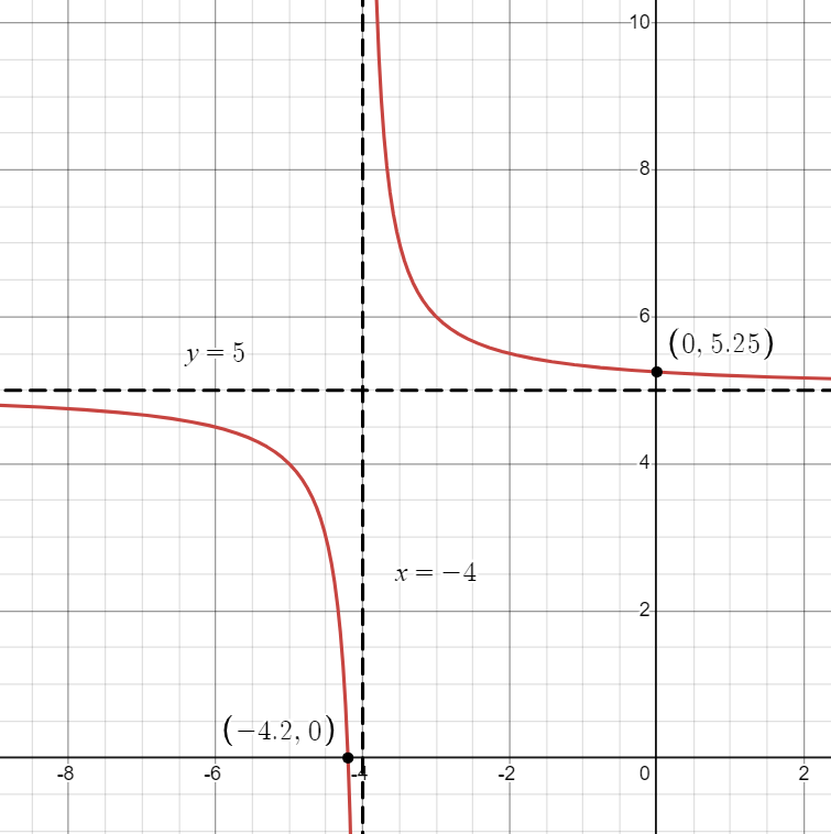
Determine the domain, range, asymptotes, intercepts, and end behaviours of \(g(x) = \cfrac{1}{x + 4} + 5\). Then, sketch a graph of the function.
First, since this function is in Standard Form, we can determine its Horizontal Asymptote as \(\boldsymbol{y = 5}\) and its Vertical Asymptote as \(\boldsymbol{x = -4}\).
Next, we can determine the function's domain. Since we have determined that the function contains a Vertical Asymptote at \(x = -4\), we can determine that the domain is restricted at this point. As a result, we can express the domain as \(\boldsymbol{\{x \in \mathbb{R} | x \neq -4\}}\).
Then, we can determine the function’s range. Since we have determined that the function contains a Horizontal Asymptote at \(x=5\), we can identify that the range is restricted at this point. As a result, we can express the range as \(\boldsymbol{\{y\in\mathbb{R} |y \ne 5\}}\).
After, we can determine the function's intercepts.
We can first determine its \(y\)-intercept by setting \(x = 0\) and solving for \(g(x)\):
\(g(0) = \cfrac{1}{0 + 4} + 5\)
\(g(0) = \cfrac{1}{4} + 5\)
\(g(0) = 0.25 + 5\)
\(g(0) = 5.25\)
Next, we can determine the \(x\)-intercept by setting \(g(x) = 0\) and solving for \(x\):
\(0 = \cfrac{1}{x + 4} + 5\)
\(-5 = \cfrac{1}{x + 4}\)
\(-5x - 20 = 1\)
\(-5x = 21\)
\(x = -4.2\)
From this, we can determine the function's \(x\) and \(y\)-intercepts are \(\boldsymbol{(0, 5.25)}\) and \(\boldsymbol{(-4.2, 0)}\) respectively.
Finally, we can determine the function’s end behaviors:
| As \(x \rightarrow\) | \(f(x) \rightarrow\) |
| \(- \infty\) | \(5\) |
| \(-4^-\) | \(-\infty\) |
| \(-4^+\) | \(+\infty\) |
| \(+ \infty\) | \(5\) |
Using the information we have determined above, we can draw a sketch of the function as such:
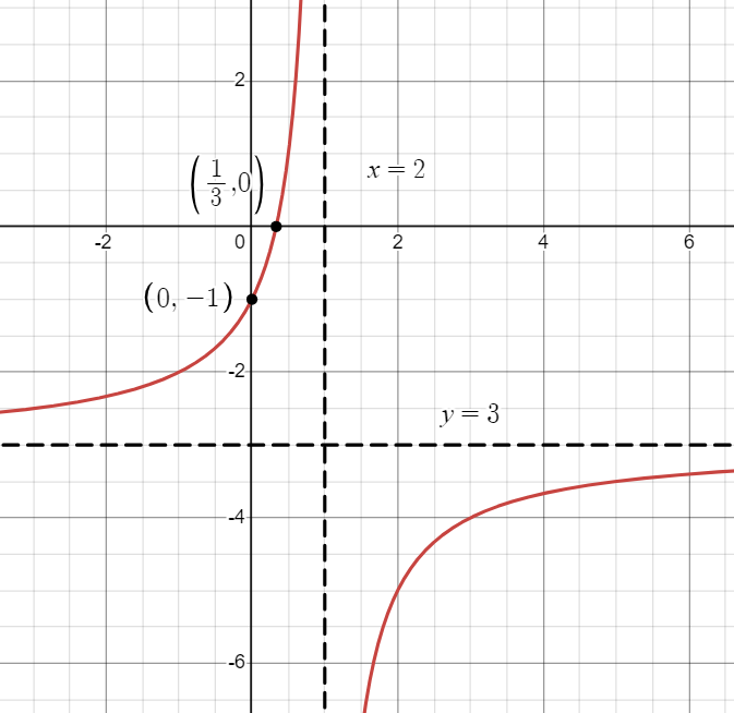
First, since this function is in Standard Form, we can determine its Horizontal Asymptote as \(\boldsymbol{y = -3}\) and its Vertical Asymptote as \(\boldsymbol{x = 1}\).
Next, we can determine the function's domain. Since we have determined that the function contains a Vertical Asymptote at \(\boldsymbol{x = 1}\), we can determine that the domain is restricted at this point. As a result, we can express the domain as \(\mathbb{\{x \in \mathbb{R} | x \neq 1\}}\).
Then, we can determine the function’s range. Since we have determined that the function contains a Horizontal Asymptote at \(x=5\), we can identify that the range is restricted at this point. As a result, we can express the range as \(\boldsymbol{\{y\in\mathbb{R} |y \ne -3\}}\).
After, we can determine the function's intercepts.
We can first determine its \(y\)-intercept by setting \(x = 0\) and solving for \(h(x)\):
\(h(0) = \cfrac{-2}{0 - 1} - 3\)
\(h(0) = \cfrac{-2}{-1} - 3\)
\(h(0) = 2 - 3\)
\(h(0) = -1\)
Next, we can determine the \(x\)-intercept by setting \(g(x) = 0\) and solving for \(x\):
\(0 = \cfrac{-2}{x - 1} - 3\)
\(3 = \cfrac{-2}{x - 1}\)
\(3x - 3 = -2\)
\(3x = 1\)
\(x = \cfrac{1}{3}\)
From this, we can determine the function's \(x\) and \(y\)-intercepts are \(\boldsymbol{(0, -1)}\) and \(\boldsymbol{\left(\cfrac{1}{3}, 0\right)}\) respectively.
Finally, we can determine the function’s end behaviors:
| As \(x \rightarrow\) | \(f(x) \rightarrow\) |
| \(- \infty\) | \(-3\) |
| \(1^-\) | \(\infty\) |
| \(1^+\) | \(-\infty\) |
| \(+ \infty\) | \(-3\) |
Using the information we have determined above, we can draw a sketch of the function as such:
Reciprocal Linear Function Calculator
Select the coefficient and term values for \(f(x)\). This function will then determine its corresponding reciprocal function and plot the \(2\) functions next to each other.