Reciprocal Quadratic Functions
A Reciprocal Quadratic Function is a reciprocal function that contains a quadratic (or second-degree polynomial) in its denominator. It can be expressed algebraically as:
Where \(k\) represents the constant value.
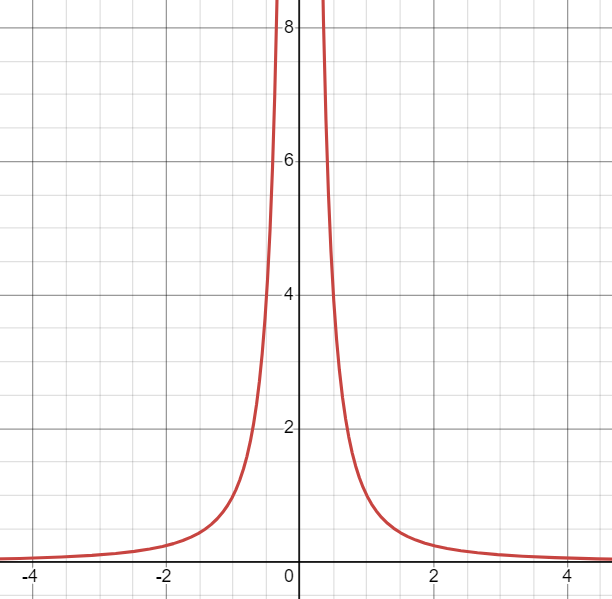
Reciprocal Quadratic Functions can be represented graphically as:
These functions can also be represented in Standard Form as:
Regular quadratic functions contain several attributes that can make graphing their reciprocal counterparts challenging. This includes their parabolic shapes, a max or min point, and a variable number of zeroes.
Characteristics of Reciprocal Quadratic Functions
Domain
The Domain of reciprocal quadratic functions is all real numbers where \(x\) cannot equal \(0\), \(\{x\in\mathbb{R}, x \ne 0)\). For functions expressed in Standard Form, the domain is limited to all real numbers where x cannot equal the Vertical Asymptotes, \(\{x\in\mathbb{R}|x\ne \text{VA's}\}\).
Range
The Range of reciprocal quadratic functions is all real numbers where \(x\) cannot equal \(0\), \(\{y\in\mathbb{R}, y \ne 0\}\). For functions expressed in Standard Form, the domain is limited to all real numbers where x cannot equal the Horizontal Asymptote (or \(d\)), \(\{y\in\mathbb{R}|y \neq d\}\).
Intercepts
The y-intercept can be determined by substituting \(0\) for \(x\) and solving for \(f(x)\). This can only be done if the function has an \(h\)-value. Otherwise, it will make the denominator \(0\), thereby making the entire function undefined.
The x-intercept(s) can be determined by setting the numerator equal to \(0\) and solving for \(x\).
Asymptotes
Vertical Asymptotes are vertical lines that a function cannot cross, thereby restricting its domain. In a reciprocal quadratic function, the roots in the denominator correspond to any of the potential vertical asymptotes. As a regular quadratic function can have either zero, one, or two vertical asymptotes, so too can its reciprocal counterpart. You can find the vertical asymptotes by factoring the denominator, then solving for \(0\) for each factor.
Horizontal Asymptotes are horizontal lines that a function approaches as its inputs, \(x\), approaches or \(-∞\). Unlike its vertical counterpart, a Horizontal Asymptote can be crossed. You can determine a horizontal asymptote by dividing each term by its highest power then evaluating \(x→∞\). If the reciprocal quadratic function is in the form \(f(x) = \cfrac{k}{ax^2 + bx + c}\), , there will always be a horizontal asymptote at \(f(x) = 0\).
Minima/Maxima
Reciprocals of quadratic functions with \(2\) Vertical Asymptotes have \(3\) parts with the middle one reaching either a minimum or maximum relative extrema. This point is equidistant from the \(2\) Vertical Asymptotes.
You can determine whether the function has a max or min point depending on the value of \(k\):
- If \(k>0\), the function will have a local maximum
- If \(k< 0\), the function will have a local minimum
The local extrema only exist for a function in the form \(f(x) = \cfrac{k}{ax^2 + bx + c}\). We can determine the value of the extrema by taking the average of the \(x\)-intercepts. We can then substitute this value into the original expression and solve.
End Behaviours
The end behavior for reciprocal quadratic functions are dependent on the k-value and are summarized in the table below assuming that \(f(x) = \cfrac{k}{x^2}\):
| k Value | Left Branch | Right Branch |
|---|---|---|
| Positive | \(x \rightarrow -\infty, y \rightarrow 0\) \(x \rightarrow 0, y \rightarrow -\infty\) | \(x \rightarrow 0, y \rightarrow +\infty\) \(x \rightarrow +\infty, y \rightarrow 0\) |
| Negative | \(x \rightarrow -\infty, y \rightarrow 0\) \(x \rightarrow 0, y \rightarrow +\infty\) | \(x \rightarrow 0, y \rightarrow -\infty\) \(x \rightarrow +\infty, y \rightarrow 0\) |
This table indicates that the end behaviors are similar regardless of \(k\)’s sign. The only difference is what \(y\) approaches on either branch when \(x\) approaches \(0\).
Outlined below are the end behaviors for reciprocal functions where \(f(x) = \cfrac{k}{(x-a)(x-b)} + d\):
| Sign | Left Branch | Middle Branch | Right Branch |
|---|---|---|---|
| Positive | \(x \rightarrow -\infty, y \rightarrow d\) \(x \rightarrow a^-, y \rightarrow +\infty\) | \(x \rightarrow a^+, y \rightarrow - \infty\) \(x \rightarrow b^-, y \rightarrow -\infty\) | \(x \rightarrow b^+, y \rightarrow +\infty\) \(x \rightarrow +\infty, y \rightarrow d\) |
| Negative | \(x \rightarrow -\infty, y \rightarrow d\) \(x \rightarrow a^-, y \rightarrow +\infty\) | \(x \rightarrow a+, y \rightarrow + \infty\) \(x \rightarrow b^-, y \rightarrow +\infty\) | \(x \rightarrow b^+, y \rightarrow -\infty\) \(x \rightarrow +\infty, y \rightarrow d\) |
Example
Determine the intercepts, domain, range, asymptotes, min/mx point and end behaviours of \(h(x) = \cfrac{1}{(x - 3)(x + 2)}\). Then, sketch a graph of the function.
First, we can determine its intercepts. We can determine that this function doesn’t contain any \(x\)-intercepts.
We can then determine its \(y\)-intercept:
\(h(0) = \cfrac{1}{(-3)(2)}\)
\(h(0) = -\cfrac{1}{6}\)
Next, we can determine the function’s asymptotes. We can start with its Vertical Asymptotes:
\(\text{VA}_1: x = 3\)
\(\text{VA}_2: x = -2\)
We can then determine its Horizontal Asymptote:
From this, we can determine the function's \(y\)-intercept is \(\boldsymbol{\left(0, -\cfrac{1}{6}\right)}\), its vertical asymptotes are \(\boldsymbol{x = -2, 3}\), and its horizontal asymptote is \(\boldsymbol{y=0}\).
After, we can determine the function’s domain. Since we have determined that the function contains vertical asymptotes at \(x=3\) and \(x=-2\), we can identify that the domain is restricted at these points. As a result, we can express the domain as \(\boldsymbol{\{x\in\mathbb{R} | x \ne 2, -3\}}\).
We can also determine that function’s range. Since we have determined that the function contains a horizontal asymptote at \(y=0\), we can identify that the range is restricted at this point. As a result, we can express the range as \(\boldsymbol{\{y\in\mathbb{R} | y \ne 0\}}\).
Additionally, we can determine the local max/min value. Since \(k>0\) in this instance, we will get a local max. We can first determine the average value of the vertical asymptotes:
\(\text{AOS}: x = \cfrac{1}{2}\)
\(\text{AOS}: x = 0.5\)
We can then substitute this value for \(x\) in the original function to get the max value:
\(h(0.5) = \cfrac{1}{(-2.5)(2.5)}\)
\(h(0.5) = -\cfrac{1}{6.25}\)
Therefore, we can determine that the max value is \(\boldsymbol{\left(0.5, -\cfrac{1}{6.25}\right)}\)
Finally, we can determine the function’s end behaviors:
| As \(x \rightarrow\) | \(f(x) \rightarrow\) |
| \(- \infty\) | \(0\) |
| \(-2^-\) | \(+\infty\) |
| \(-2^+\) | \(-\infty\) |
| \(3^-\) | \(-\infty\) |
| \(3^+\) | \(+\infty\) |
| \(+ \infty\) | \(0\) |
Using the information we have determined above, we can draw a sketch of the function as such:
![Graph of transformed Reciprocal Quadratic Function with equation h(x)=1/[(x-3)(x+2)]](RationalQuads2.PNG)
First, we can determine its intercepts. We can determine that this function doesn’t contain any \(x\)-intercepts.
We can then determine its \(y\)-intercept:
\(i(0) = \cfrac{-5}{(7)(4)}\)
\(i(0) = \cfrac{-5}{28}\)
Next, we can determine the function’s asymptotes. We can start with its Vertical Asymptotes:
\(\text{VA}_1: x = -4\)
\(\text{VA}_2: x = -7\)
We can then determine its Horizontal Asymptote:
From this, we can determine the function's \(y\)-intercept is \(\boldsymbol{\left(0, \cfrac{-5}{28}\right)}\), its vertical asymptotes are \(x= -7, -4\), and its horizontal asymptote is \(\boldsymbol{y = 0}\).
After, we can determine the function’s domain. Since we have determined that the function contains vertical asymptotes at \(x=-4\) and \(x=-7\), we can identify that the domain is restricted at these points. As a result, we can express the domain as \(\boldsymbol{\{x\in\mathbb{R} | x \ne -4, -7\}}\).
We can also determine that function’s range. Since we have determined that the function contains a horizontal asymptote at \(y=0\), we can identify that the range is restricted at this point. As a result, we can express the range as \(\boldsymbol{\{y\in\mathbb{R} | y \ne 0\}}\).
Additionally, we can determine the local max/min value. Since \(k< 0\) in this instance, we will get a local min. We can first determine the average value of the vertical asymptotes:
\(\text{AOS}: x = \cfrac{-11}{2}\)
\(\text{AOS}: x= -5.5\)
We can then substitute this value for \(x\) in the original function to get the max value:
\(h(-5.5) = \cfrac{-5}{(1.5)(-1.5)}\)
\(h(-5.5) = \cfrac{-5}{-2.25}\)
\(h(-5.5) = \cfrac{1}{0.45}\)
Therefore, we can determine that the min value is \(\boldsymbol{\left(-5.5, \cfrac{1}{0.45}\right)}\)
Finally, we can determine the function’s end behaviors:
| As \(x \rightarrow\) | \(f(x) \rightarrow\) |
| \(- \infty\) | \(0\) |
| \(-7^-\) | \(-\infty\) |
| \(-7^+\) | \(+\infty\) |
| \(-4^-\) | \(+\infty\) |
| \(-4^+\) | \(-\infty\) |
| \(+ \infty\) | \(0\) |
Using the information we have determined above, we can draw a sketch of the function as such:
![Graph of transformed Reciprocal Quadratic Function with equation -2/[(x+7)(x+4)].](RationalQuads3.PNG)