Word Problems
The equation \(A(t) = 100\left(\cfrac{1}{2}\right)^{\mathord{\frac{t}{250}}}\) was used to find the present-day radioactivity of some wooden tools at an archaeological dig.
- What do each of the variables represent?
- Find the percent of radiation left after \(1000\) years.
- Fill in the table below.
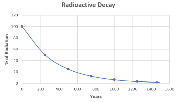
- Sketch a graph of this function.
| Years | 0 | 250 | 500 | |||
|---|---|---|---|---|---|---|
| % of Radiation | 100 |
i. We can identify what each variable and value as such:
- \(A\) represents the final amount of radiation
- \(100\) represents the initial % of radiation
- \(1/2\) represents the decay rate (half-life)
- \(t\) represents time in years
- \(250\) represents the time it takes to decay by half
ii. We can plug the # of years (\(1000\)) into the formula to determine the % of radiation left after that time:
\(A(1000) = 100\left(\cfrac{1}{2}\right)^{\frac{1000}{250}}\)
\(A(1000) = 100\left(\cfrac{1}{2}\right)^4\)
\(A(1000) = 100\left(\cfrac{1}{16}\right)\)
\(A(1000) = 6.25\)
Therefore, we can determine that there will be \(\boldsymbol{6.25 \%}\) of radiation left after \(1000\) years.
iii. We can use the formula to fill in the rest of the table. We will determine the % of radiation left in 250 year periods ending with \(1250\):
We can first determine the radiation percentage at \(250\) years:
\(A(250) = 100\left(\cfrac{1}{2}\right)^{\frac{250}{250}}\)
\(A(250) = 100\left(\cfrac{1}{2}\right)^1\)
\(A(250) = 100\left(\cfrac{1}{2}\right)\)
\(A(250) = 50\)
We can then determine the radiation percentage at \(500\) years:
\(A(500) = 100\left(\cfrac{1}{2}\right)^{\frac{500}{250}}\)
\(A(500) = 100\left(\cfrac{1}{2}\right)^2\)
\(A(500) = 100\left(\cfrac{1}{4}\right)\)
\(A(500) = 25\)
We can then determine the radiation percentage at \(750\) years:
\(A(750) = 100\left(\cfrac{1}{2}\right)^{\frac{750}{250}}\)
\(A(750) = 100\left(\cfrac{1}{2}\right)^3\)
\(A(750) = 100\left(\cfrac{1}{8}\right)\)
\(A(750) = 12.5\)
We can then determine the radiation percentage at \(1250\) years:
\(A(1250) = 100\left(\cfrac{1}{2}\right)^{\frac{1250}{250}}\)
\(A(1250) = 100\left(\cfrac{1}{2}\right)^5\)
\(A(1250) = 100\left(\cfrac{1}{32}\right)\)
\(A(1250) = 3.125\)
Note: We didn't have to solve for \(t = 1000\) above as we already did in the last part.
| Years | 0 | 250 | 500 | 750 | 1000 | 1250 |
|---|---|---|---|---|---|---|
| % of Radiation | 100 | 50 | 25 | 12.5 | 6.25 | 3.125 |
iv. We can use our table of values as a reference for sketching our graph:
Deprecation is the decline in a car's value over the course of its useful life. Most modern domestic vehicles typically deprecate at a rate of \(15-20\%\) per year depending on the model of the car. A 2007 Ford Mustang convertible is valued at \($32000\) and deprecates on average at \(20\%\) per year.
- Find an equation that will model this relationship
- Fill in the table below
- How much value will the car lose in the 1st year?
- How much value does the car lose in the 5th year?
- After how many years will the value of the car be half of the original purchase price?
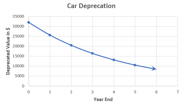
- Sketch a graph of this function
| Year End | 0 | 1 | 2 | 3 | 4 | 5 |
|---|---|---|---|---|---|---|
| Value in $ | 32000 |
i. In order to determine the formula, we can first identify what each variable and value represents:
- \(V(y)\) represents the value of the car after each year
- \(32000\) represents the initital amount
- \(0.2\) represents the deprecation rate
- \(1-0.2\) (or \(0.8\)) represents the deprecation factor
- \(y\) represents the period in time in years where the car deprecates in value
Using this information, we can now set up our formula:
Therefore, we can determine that the formula is \(\boldsymbol{V(y) = 32000(0.8)^y}\).
ii. We can use the formula we determined above to fill in the rest of the table:
We can first determine the dollar value after \(1\) year:
\(V(1) = 32000(0.8)^1\)
\(V(1) = 32000(0.8)\)
\(V(1) = 25600\)
We can then determine the dollar value after \(2\) years:
\(V(2) = 32000(0.8)^2\)
\(V(2) = 32000(0.64)\)
\(V(2) = 20480\)
We can then determine the dollar value after \(3\) years:
\(V(3) = 32000(0.8)^3\)
\(V(3) = 32000(0.512)\)
\(V(3) = 16384\)
We can then determine the dollar value after \(4\) years:
\(V(4) = 32000(0.8)^4\)
\(V(4) = 32000(0.4096)\)
\(V(4) = 13107.2\)
We can then determine the dollar value after \(5\) years:
\(V(5) = 32000(0.8)^5\)
\(V(5) = 32000(0.32768)\)
\(V(5) = 10485.76\)
| Year End | 0 | 1 | 2 | 3 | 4 | 5 |
|---|---|---|---|---|---|---|
| Value in $ | 32000 | 25600 | 20480 | 16384 | 13107.2 | 10485.76 |
iii. We can determine how much value the car lost in the first year by subtracting the initial value (\($32000\)) by value after the first year (\($25600\)):
\(\text{Lost}_1 = $32000 - $25600\)
\(\text{Lost}_1 = $6400\)
Therefore, we can determine that the car lost \(\boldsymbol{$6400}\) in value within the first year.
iv. We can determine how much value car lost in the fifth year by subtracting the car's value after the fourth year (\($13107.2\)) by value after the fifth year (\($10485.76\))
\(\text{Lost}_5 = $13107.2 - $10485.76\)
\(\text{Lost}_5 = $2621.44\)
Therefore, we can determine that the car lost \(\boldsymbol{$2621.44}\) in value within the fifth year.
v. In order to determine when the car will reach half of its initial value (\($16000\)), we can use our graph for reference. In doing so, we can identify that it will reach this point after 3-4 years.
We can also use logarithms in order to more accurately identify when it will reach this point:
\(16000 = 32000(0.8)^y\)
\(\cfrac{16000}{32000} = \cfrac{32000(0.8)^y}{32000}\)
\(0.5 = (0.8)^y\)
\(y(\text{log}(0.8)) = \text{log}(0.5)\)
\(y = \cfrac{-0.301029995}{-0.096910013}\)
\(y = 3.106283713 \approx 3.11\)
Therefore, we can accurately determine that the car will reach have its initial value after roughly \(\boldsymbol{3.11}\) years.
vi. We can use our table of values as a reference for sketching our graph:
The population of a bacteria culture is cut in half by an antibitotic every \(30\) minutes.
- If the entire bacteria culture is present at \(5 \colon 00\; [\text{a.m.}]\), what fraction of the bacteria culture will be left at \(9 \colon 30 [\text{a.m.}]\)?
- At what time will the bacteria culture contain \(\cfrac{1}{128}\) of its original population?
i. First we can identify what each variable and value represents:
- \(B(m)\) represents how much bacteria remains after a certain period of time
- \(1\) represents the inital amount since the entire bacteria culture exists at the beginning of the time frame
- \(1/2\) represents the Decay Factor
- \(m\) represents the time in minutes
- \(30\) represents how often the bacteria culture is cut in half
- \(270\) represents the amount of time in minutes between the start and end times
Next, we can set up our formula using these variables and values and determine the remainder of the bacteria culture at the end time:
\(B(m) = 1\left(\cfrac{1}{2}\right)^{\frac{m}{30}}\)
\(B(270) = 1\left(\cfrac{1}{2}\right)^{\frac{270}{30}}\)
\(B(270) = 1\left(\cfrac{1}{2}\right)^9\)
\(B(270) = \cfrac{1}{512}\)
\(B(270) = 0.1955\)
Therefore, we can determine that roughly \(\boldsymbol{0.195 \%}\) of the bacteria population remains at \(9 \colon 30\; [\text{a.m}]\).
ii. First, we can set up our formula similar to how we did in the first part:
In order to determine the # of minutes since the start time, we can either use trial and error or logarithms. We will show how to accomplish this using the latter technique:
\(\text{log}\left(\cfrac{1}{128}\right) = \left(\cfrac{m}{30}\right)\left(\text{log}\left(\cfrac{1}{2}\right)\right)\)
\(\cfrac{m}{30} = \cfrac{\text{log}\left(\cfrac{1}{128}\right)}{\text{log}\left(\cfrac{1}{2}\right)}\)
\(\cfrac{m}{30} = \cfrac{-2.10720997}{-0.301029995}\)
\(\cfrac{m}{30} = 7\)
\(m = 210\)
\(m = 3\;[\text{h}] \; 30\;[\text{min}]\)
We can now add the # of minutes to the start time to get our result:
\(T = 5 \colon 30\;[\text{a.m.}] + 3\;[\text{h}] \; 30\; [\text{min}]\)
\(T = 8 \colon 30\;[\text{a.m.}]\)
Therefore, we can determine that the bacteria culture will contain \(\boldsymbol{\cfrac{1}{128}}\) of its original population at \(8 \colon 30 \; [\text{a.m.}]\).