Exponential Functions
Exponential Functions are mathematical functions used in several real-world applications, primarily Exponential Growth and Decay. They are normally expressed as such:
- \(f(x)\) represents the dependent variable
- \(x\) represents the independent variable
- \(a\) represents the vertical stretch/compression factor
- \(b\) represents the Growth/Decay factor
- \(c\) represents the vertical shift

Unlike Linear Functions which change at a constant rate, Exponential Functions change by a common ratio.
NOTE: In an exponential, \(a > 0\). Otherwise, this will result in an error! In addition, \(a \ne 1\) since \(1\) exponentiated by any value is still \(1\).
Characteristics of Exponentials
Growth/Decay Factor
The Growth/Decay Factor, \(b\), is used to determine whether the quantity rapidly increases or decreases. This can be found by identifying the Growth/Decay Rate, \(r\); this value gets added to or modifies \(b\).
These factor changes can be expressed as:- % Increase: \(b = 1 + r\)
- % Decrease: \(b = 1 - r\)
Regarding growth, if a quantity were to double in value each period, \(b = 2\). Likewise, if a quantity were to increase by 5% each period, \(b = 1.05\).
Conversely, regarding decay in relation to half-life, \(b = 0.5\). Similarly, if a quantity were to decrease by 8% each period, \(b = 0.92\).
Horizontal Aymptote
The Horizontal Asymptote is the horizontal portion of the graph which the function approaches but never actually touches.
- An exponential function has a default H.A of \(y = 0\)
- If the exponential is vertically shifted by a value of \(c\), then the H.A will become \(y = c\)
Domain
- The Domain is defined by default as \(\{x\in\mathbb{R}\}\) meaning that it consists of all real numbers
- The Domain will remain constant regardless of any transformations applied to the parent function
Range
- The Range is defined by default as \(\{y\in\mathbb{R} |y > 0\}\) meaning that it consists of all real numbers greater than \(0\).
- The function will always be greater or less than the value of the horizontal asymptote depending on what transformations are applied to the parent
- If the parent function is vertically shifted by a value of \(c\), the Range will change to \(\{y\in\mathbb{R} | y > c\}\)
- If the parent function is flipped horizontally, the Range will change to \(\{y\in\mathbb{R} | y < c\}\)
y-intercept
- The point where the parabola crosses the y-axis
- Can be determined algebraically by setting \(x = 0\) in the exponential function
- If no transformations are applied to the function, the y-int will always be 1
Example
For the function \(f(x) = 3^x\):
- Sketch a graph
- Determine the Domain, Range, Intercepts, and Horizontal Asymptote
i. In order to draw our graph, we can first create a table of values:
| x Values | -3 | -2 | -1 | 0 | 1 | 2 | 3 |
|---|---|---|---|---|---|---|---|
| y Values | 0.037 | 0.11 | 0.33 | 1 | 3 | 9 | 27 |
Using this table of values, we can create our graph:

ii. By looking at our graph, we can determine the following:
- Domain: \(\boldsymbol{\{x∈ℝ\}}\)
- Range: \(\boldsymbol{\{y∈ℝ |y > 0\}}\)
- Intercepts: \(\boldsymbol{y = 1}\)
- H.A: \(\boldsymbol{y = 0}\)
For the following functions:
- Sketch a graph.
- Determine the Domain, Range, Intercepts, and Horizontal Asymptote.
\(h(x) = \left(\cfrac{1}{2}\right)^x+2\)
i. In order to draw our graph, we can first create a table of values:
| x Values | -3 | -2 | -1 | 0 | 1 | 2 | 3 |
|---|---|---|---|---|---|---|---|
| y Values | 10 | 6 | 4 | 3 | 2.5 | 2.25 | 2.125 |
Using this table of values, we can create our graph:
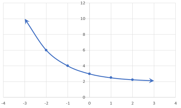
ii. By looking at our graph, we can determine the following:
- Domain: \(\boldsymbol{\{x\in\mathbb{R}\}}\)
- Range: \(\boldsymbol{\{y\in\mathbb{R} |y > 2\}}\)
- Intercepts: \(\boldsymbol{y = 3}\)
- H.A: \(\boldsymbol{y = 2}\)
\(g(x) = -(2.5)^x-5\)
i. In order to draw our graph, we can first create a table of values:
| x Values | -3 | -2 | -1 | 0 | 1 | 2 | 3 |
|---|---|---|---|---|---|---|---|
| y Values | -5.064 | -5.16 | -5.4 | -6 | -7.5 | -11.25 | -20.625 |
Using this table of values, we can create our graph:
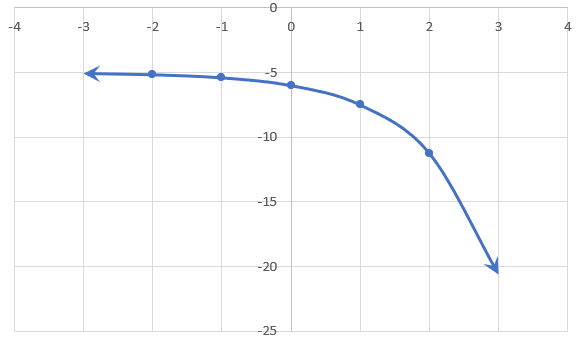
ii. By looking at our graph, we can determine the following:
- Domain: \(\boldsymbol{\{x\in\mathbb{R}\}}\)
- Range: \(\boldsymbol{\{y\in\mathbb{R} |y < 5\}}\)
- Intercepts: \(\boldsymbol{y = 5}\)
- H.A: \(\boldsymbol{y = -6}\)
Writing Equations of Exponential Functions
Using tables of values or graphs, we can to determine the equations for exponential functions:
Steps
- Determine if there is a Horizontal Asymptote to use as the \(c\) value
- Use a pair of coordinates to create 2 different equations
- Divide the second equation by the first equation to solve for \(b\)
- Substitute the \(b\) value into either of the equations to solve for \(a\)
- Put all the variables together to get the final equation
Example
Determine the equation of the following function using the following table of values and the Horizontal Asymptote:
| x Values | -1 | 0 | 1 | 2 | 3 | 4 | 5 |
|---|---|---|---|---|---|---|---|
| y Values | 168 | 84 | 42 | 21 | 10.5 | 5.25 | 2.625 |
Horizontal Asymptote: \(y = 0\)
First, we can determine that there is no real \(c\) value since the H.A is \(0\).
Next, we can create our 2 equations using the table of values. In this case, we will use the value pairs for \(x = -1\) and \(x = 0\) respectively:
\(f(x) = ab^x + 0\)
\(f(-1) = ab^{-1} = 168\)
\(f(0) = ab^0 = 84\)
Then, we can divide equation 2 by equation 1. Since the \(a\)'s will cancel out, this will allow us to solve for \(b\):
\(\cfrac{f(0)}{f(-1)}\)
\(\cfrac{ab^0 = 84}{ab^{-1} = 168}\)
\(\cfrac{\cancel{a}b^0}{\cancel{a}b^{-1}} = 0.5\)
\(b = 0.5\)
After, we can substitute \(0.5\) for \(b\) in either of the equations we used in the previous step to solve for \(a\). In this instance, we will use Equation 1:
\(168 = ab^{-1}\)
\(a(0.5)^{-1} = 168\)
\(\cfrac{2a}{2} = \cfrac{168}{2}\)
\(a = 84\)
Finally, we can put all the variables together to get our final equation:
Therefore, we can determine that the equation for this table of values is \(\boldsymbol{f(x) = 84(0.5)^x}\).
| x Values | 3 | 6 | 9 | 12 | 15 | 18 |
|---|---|---|---|---|---|---|
| y Values | 17.49783 | 71.6182 | 314.7336 | 1406.839 | 6312.711 | 28350.5 |
Horizontal Asymptote: \(y = 2\)
First, we can determine that \(c = 2\).
Next, we can create our 2 equations using the table of values. We can use the following formula as a reference:
In this case, we will use the value pairs for \(x = 3\) and \(x = 6\) respectively. We will also round the \(y\)-values to one decimal place.
We can determine the first equation as such:
\(f(3) = ab^{3} + 2 = 17.5\)
\(f(3) = ab^{3} = 17.5 - 2\)
\(f(3) = ab^{3} = 15.5\)
We can determine the second equation as such:
\(f(6) = ab^6 + 2 = 71.6\)
\(f(6) = ab^6 = 71.6 - 2\)
\(f(6) = ab^6 = 69.6\)
Then, we can divide Equation 2 by Equation 1. Since the \(a\)'s will cancel out, this will allow us to solve for \(b\):
\(\cfrac{f(6)}{f(3)}\)
\(\cfrac{ab^6 = 69.6}{ab^3 = 15.5 }\)
\(\cfrac{\cancel{a}b^{6-3}}{\cancel{a}} = 4.49\)
\(b^3 = 4.49\)
\(\sqrt[3]{b^3} = \sqrt[3]{4.49}\)
\(b = 1.65\)
After, we can substitute 1.65 for \(b\) in either of the equations we used in the previous step to solve for \(a\). In this instance, we will use Equation 1:
\(ab^3 = 15.5\)
\(a(1.65)^3 = 15.5\)
\(\cfrac{4.49a}{4.49} = \cfrac{15.5}{4.49}\)
\(a = 3.45\)
Finally, we can put all the variables together to get our final equation:
Therefore, we can determine that the equation for this table of values is \(\boldsymbol{f(x) = 3.45(1.65)^x + 2}\).
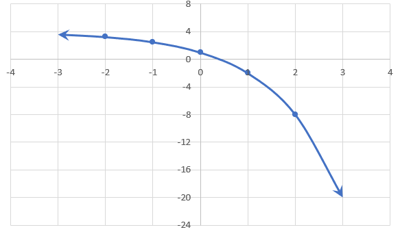
First, we can determine from looking at the graph that \(c = 4\) since that is where the function approaches but doesn't touch.
Next, we can create our 2 equations using the graph. We can use the following formula as a reference:
In this case, we will use the pairs \((1, -2)\) and \((2, -8)\) to determine our equations.
We can determine the first equation as such:
\(f(1) = ab^1 + 4 = -2\)
\(f(1) = ab^1 = -2 - 4\)
\(f(1) = ab^1 = -6\)
We can determine the second equation as such:
\(f(2) = ab^2 + 4 = -8\)
\(f(2) = ab^2 = -8 - 4\)
\(f(2) = ab^2 = -12\)
Then, we can divide Equation 2 by Equation 1 to solve for \(b\):
\(\cfrac{f(2)}{f(1)}\)
\(\cfrac{ab^2 = -12}{ab^1 = -6}\)
\(\cfrac{\cancel{a}b^{2-1}}{\cancel{a}} = 2\)
\(b = 2\)
After, we can substitute \(2\) for \(b\) in either of the equations we used in the previous step to solve for \(a\). In this instance, we will use Equation 1:
\(ab^1 = -6\)
\(a(2)^1 = -6\)
\(\cfrac{2a}{2} = \cfrac{-6}{2}\)
\(a = -3\)
Finally, we can put all the variables together to get our final equation:
Therefore, we can determine that the equation for this table of values is \(\boldsymbol{f(x) = -3(2)^x + 4}\).