Linear Relationships
A Linear Relationship is used to describe a straight-line (or direction) relation between two variables. It can be expressed as a table of values or a graph where the data points are connected via a straight line. This includes vertical and horizontal lines.
Mathematically, a linear relationship is one that satisfies the equation:
\(y = m(x) + b\)
where \(m\) is the slope and \(b\) is the \(y\)-intercept. Recall the slope formula is the change in \(y\) over change in \(x\).
Table of Values
Every linear equation is a relationship of \(x\) and \(y\)-values. To create a table of values, we just have to pick a set of \(x\) values, substitute them into the equation and evaluate to get the \(y\)-values. You could also read the points from a graph.
Enter the slope and \(y\)-intercept below to create a table of values.
First Differences
The First Differences are the differences between consecutive \(y\)-values in tables of values with evenly spaced \(x\)-values. When the first difference is constant (the same), the relation is linear.
For example, Jameen has recorded his sleep for the week in the table below.
| x (Day) | Mon | Tues | Wed | Thur | Fri | Sat | Sun |
|---|---|---|---|---|---|---|---|
| y (Hours) | 8 | 10 | 11 | 9 | 12 | 9 | 10 |
To calculate the first difference, we can subtract the second \(y\)-value form the first:
We can continue with this process with the remaining \(y\)-values to determine whether the relationship is linear or non-linear.
The difference in the \(y\)-values are \(2,1,-2,3,-3,1\). Thus, we can determine that the relationship of Jameen's sleep is non-linear.
| x Values | 0 | 1 | 2 | 3 | 4 | 5 |
|---|---|---|---|---|---|---|
| y Values | 10 | 13 | 16 | 19 | 22 | 25 |
First, we can notice that the \(x\)-values are evenly spaced and increase by \(1\).
Next, we can calculate the difference in \(y\)-values to determine whether the relationship is linear or non-linear. We can start with calculating the difference between the first \(2\) \(y\)-values:
We can continue this process for the remaining \(y\)-values. We can record the differences in a table to identify the relationship:
| x Values | 0 | 1 | 2 | 3 | 4 | 5 |
|---|---|---|---|---|---|---|
| y Values | 10 | 13 | 16 | 19 | 22 | 25 |
| 1st Diff | - | 3 | 3 | 3 | 3 | 3 |
As observed from the table, the \(y\)-value increases by \(3\) for every value increased in \(x\). Since the first differences are constant, this indicates that this relationship is linear.
Scatter Plots
A Scatter Plot shows the relationship between two variables on a graph. The values of one variable appear on the horizontal axis (independent variable, typically \(x\)), and the values of the other variable appear on the vertical axis (dependent variable, typically \(y\)).
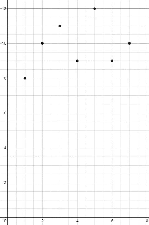
For example, Jameen has recorded his sleep for the week. The data can also be presented on a graph.
| x (Day) | Mon | Tues | Wed | Thur | Fri | Sat | Sun |
|---|---|---|---|---|---|---|---|
| y (Hours) | 8 | 10 | 11 | 9 | 12 | 9 | 10 |
We can represent this data graphically as such:
Linear vs Non-Linear Relationships
A scatter plot can be used to identify several different types of relationships between two variables.
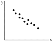
- The relationship is linear when the points on a scatter plot follow a somewhat straight line pattern.
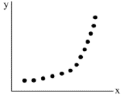
- The relationship is considered non-linear if the points on a scatter plot follow a pattern but not a straight line
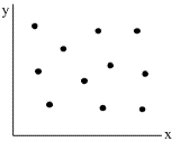
- The relationship has no correlation if the points on the scatter plot do not show any pattern.
Linear
Non-Linear
No-Correlation
An outlier is a data point that does not follow the general trend.
Direct vs Indirect Variation
Two variables vary directly (Direct Variation) if they are directly proportional to each other. The relation would have the form \(y = m(x)\) (i.e., \(b=0\)) and the graph passes through the origin \((0,0)\).
A Partial Variation is one where the the value of the dependent variable depends on both the value of the independent variable and some initial value. they are the form \(y = mx + b \) and the graph never passes through the origin \((0,0)\).
In turn, a variation is inverse if \(y\) is expressed as the product of some constant number \(k\) and the reciprocal of \(x\), given that \(k \ne 0\).
| Direct Variation | Indirect Variation | Inverse Variation |
|---|---|---|
| \(y=2.5x\) | \(y=2.5x+4\) | \(y=\cfrac{1}{x}\) |
| \(y=\cfrac{1}{2}x\) | \(y=\cfrac{3}{2}x-1/5\) | \(y=\cfrac{-3}{x}\) |
| \(y=x\) | \(y=x-1\) | \(y=\cfrac{5}{x}\) |
Example
A train can travel \(500\) kilometers within \(4\) hours.
- Determine the constant of variation
- Calculate the train's distance after \(7\) hours
i. This relation can be expressed as:
\(d=kt\)
where \(d\) represents the distance and \(t\) represents the time.
In order to determine \(k\), we can rearrange the formula in terms of \(k\) and plug in the appropriate values to solve for the constant of variation:
\(k = \cfrac{d}{t}\)
\(k = \cfrac{500}{4}\)
\(k = 125\)
Therefore, we can determine the constant of variation is \(\boldsymbol{125 \; [\textbf{km/h}]}\).
ii. Given we have determined the constant of variation, we can express this relation as such:
In order to determine the train's distance after \(7\) hours, we can substitute \(7\) into the equation and solve:
\(d=125(7)\)
\(d=875\)
Therefore, we can determine that the train will have travelled \(\boldsymbol{875 \; [\textbf{km}]}\) after \(7 \; [\text{h}]\).
The total cost, \(C\) of meat in dollars varies directly with its mass, \(m\) in kilograms.
- Find an equation relating \(C\) and \(m\) if a \(15 \;[\text{kg}]\) piece of meat costs \($4.50 [\text{s}]\)
- Use the equation to determine the total cost of the meat if it weights \(70 \;[\text{kg}]\)
i. First, we can express this relation as:
\(C = km\)
We can then rearrange this formula in terms of \(k\) and substitute the pertinent values to solve for the constant of variation:
\(k = \cfrac{C}{m}\)
\(k = \cfrac{4.50}{15}\)
\(k = 0.30\)
Since we can determine \(k = 0.30\), we can write the equation as such:
\(\boldsymbol{C = 0.3m}\)
ii. We can determine the total cost of \(70 \;[\text{kg}]\) meat by subtituting this value into the formula and solving:
\(C = 0.3(70)\)
\(C = 2.1\)
Therefore, we can determine that the \(70 \;[\text{kg}]\) meat costs \(\boldsymbol{$2.10}\).
Example
For the following table:
| x Values | 0 | 1 | 2 | 3 | 4 | |
|---|---|---|---|---|---|---|
| y Values | 3 | 5 | 9 | 21 |
- Complete the table of values given that \(y\) varies partially with \(x\).
- Identify the initial value of \(y\) and the constant of variation from the completed table. Write an equation relating \(y\) and \(x\) in the form \(y=mx+b\).
- Graph this relation.
- Describe the graph.
i. Using First Differences, we can determine that as \(x\) changes from \(0\) to \(1\), \(y\) changes from \(3\) to \(5\). Therefore, \(y\) increases by \(3\) as \(x\) increases by \(1\).
| x Values | 0 | 1 | 2 | 3 | 4 | 9 |
|---|---|---|---|---|---|---|
| y Values | 3 | 5 | 7 | 9 | 11 | 21 |
ii. The initial value of \(y\) occurs when \(x=0\). The initial value of \(y\) is \(3\). As \(x\) increases by \(1\), \(y\) increases by \(2\). Therefore, the constant of variation is \(2\).
Using this information, we can write the equation as such:
\(\boldsymbol{y = 2x + 3}\)
iii. We can graph this relation as such:

iv. The graph is a straight line the intersects the \(y\)-axis at the point \((0, 3)\). The \(y\)-values increase by \(2\) as the \(x\)-values increase by \(1\).
A shoe salesman makes a basic income of \($100\)/week plus \(4\)% of total sales.
- Identify the fixed income and the variable income of this partial variation.
- Determine the equation relating the income, \(I\), in dollars, and the number of sales, \(n\).
- Use the equation to determine the weekly income of a salesman who makes \(200\) sales a within that time.
i. Based on the question description, we can determine the fixed income as \(\boldsymbol{100}\) and the variable income as \(\boldsymbol{0.04}\).
ii. We can write the equation representing the salesman's total income as such:
\(\boldsymbol{I = 0.04n + 100}\)
iii. We can substitute \(n = 20\) into the formula and solve:
\(I = 0.04(200) + 100\)
\(I = 8 + 100\)
\(I = 108\)
Therefore, we can determine that the salesman makes \(\boldsymbol{$108}\) if they sell \(200\) shoes.
Rule of Four
A relation can be represented in a variety of ways so that it can be looked at from different points of view. A mathematical relation can be described in four ways:
- Using Words
- Using a Diagram or Graph
- Using Numbers
- Using an Equation