Interpolation and Extrapolation
We use graphs to visualize trends between variables. We can use the trend to make predictions about other data points not available. When the predictable data falls within the available data points it is called interpolation. When the data falls outside the available data points it is called extrapolation.
Line of Best Fit
A Line of Best Fit simply refers to a line drawn through a scatter plot of data points that best expresses the relationship between those points.
To draw the line of best fit, we can estimated by drawing a line through most of the data points. However, there also exist a way to calculate the actual best line using Least Squares Regression (learnt later).
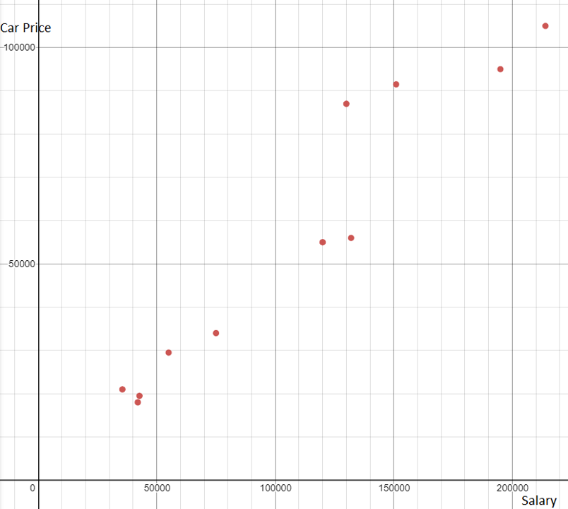
The table below shows the annual salaries of consumers and the price of cars they drive (in thousands of dollars):
| x Values(Salary, k$) | 42.7 | 195.0 | 35.5 | 214.0 | 75.0 | 130.0 | 42.0 | 151.0 | 55.0 | 120.0 | 132.0 |
|---|---|---|---|---|---|---|---|---|---|---|---|
| y Values (Car price, k$) | 19.5 | 95.0 | 21.0 | 105.0 | 34.0 | 87.0 | 18.0 | 91.5 | 29.5 | 55.0 | 56.0 |
By plotting the points on a graph, we see there is a linear positive relation between the salary and cost of the car. That means, in general, someone who makes more money will have a more expensive car.
We can draw a line of best fit through the data that shows the trend between the two variables. The line should go through many points and be close to the others.

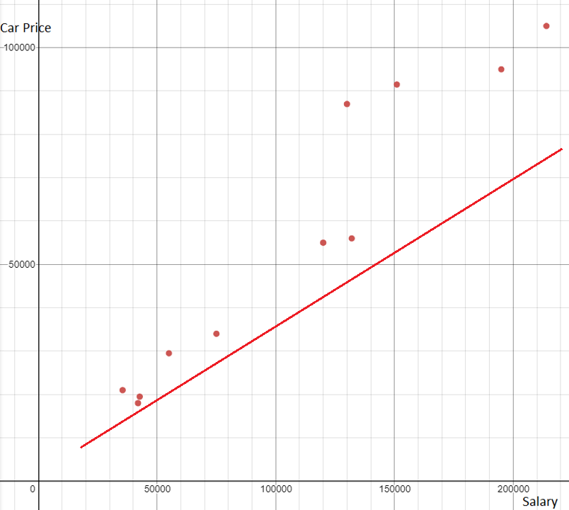
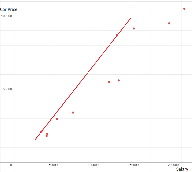
Let's look at some not so good lines of best fit. The first line doesn't go through any of the points. The second line goes through two points but is far away from the others.
A tip for drawing a good line of best fit is to make sure the number of points above and below the line are similar.
An outlier refers to a point that is separated from the main body of data on a graph. Sometimes, an outlier results from a meaurement error or from some factor that affects only a few of the observed values for a variable. In a scatter plot, an outlier is a point that either doesn't touch or is far away from the line of best fit.
First, let's estimate two points on the line. Try to pick numbers that are easy to estimate that lie near the grid of the plot:
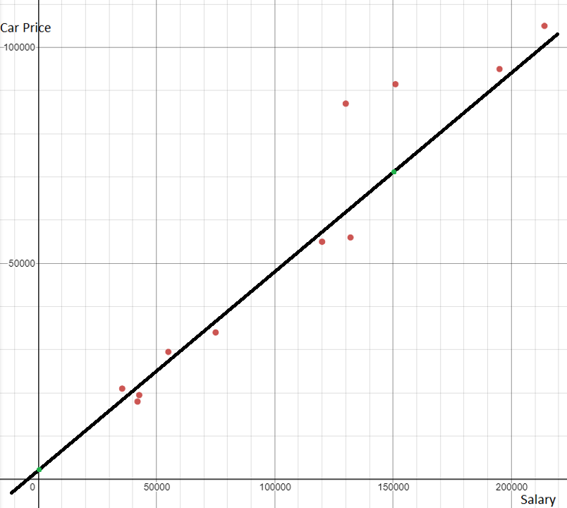
In this instance, we will choose \((0, 2,000)\) and \((150,000, 71,000)\) as our two points.
From these two points we can find the approximate slope:
\(m = \cfrac{y_2 - y_1}{x_2 - x_1}\)
\(m = \cfrac{71,000-2,000}{150,000-0} \)
\(m = \cfrac{69,000}{150,000} \)
\(m = 0.46\)
Next, we need to determine the \(y\)-intercept. We already estimate the \(y\)-intercept as one of the points, \((0, 2,000)\).
Then, we substitute in the values and can write the equation as such:
\(y = 0.46x + 2000\)
Therefore, we have determined the equation for the line of best fit as \(\boldsymbol{y = 0.46x + 2000}\)!
Interpolating
Notice we do not have a data point at a salary at \($80,000\). Instead, we can use the line of best fit to estimate the price of the car.
We have determined the equation for the line of best fit from the previous question:
\(y = 0.46x + 2000\)
Next, we can substitute \(80,000\) for \(x\) and solve:
\( y = 0.46(80000) +2000 \)
\(y = $38,800\)
From within the graph, the estimated price of cars for consumers making \($80,000\) to drive would be worth around \(\boldsymbol{$38,8000}\). Check if this looks right by plotting the point on the graph!
Extrapolating
We have determined the equation for the line of best fit from the previous question:
\(y = 0.46x + 2000\)
Next, we can aubstitute \(1,000,000\) for \(x\) and solve:
\( y = 0.46(1000000) +2000 \)
\(y = $462,000\)
Predicting outside the graph, the estimated price of cars for consumers making \($1\) million to drive would be worth around \(\boldsymbol{$462,000}\).
Be careful when extrapolating! You never know if the trend will continue outside the data we have.