Transformations of Functions
As stated previously, several transformations can be applied to parent functions in order to change their core attributes. These include:
- \(a\) represents the vertical stretch/compression factor.
- \(k\) represents the horizontal stretch/compression factor
- \(d\) represents the horizontal shift
- \(c\) represents the vertical shift
Vertical Stretch/Compression
The value of \(a\) will determine whether the transformed function will be vertically stretched or compressed:
- If \(a > 1\), the function will be vertically stretched
- If \(0 < a < 1\), the function will be vertically compressed
- If \(a < 0\), the function will either be vertically stretched or compressed with a reflection in the \(x\)-axis
Horizontal Stretch/Compression
The value of \(k\) will determine whether the transformed function will be horizontally stretched or compressed:
- If \(0 < k < 1\), the function will be horizontally stretched by a factor of \(1/k\)
- If \(k > 1\), the function will be horizontally compressed by a factor of \(1/k\)
- If \(k < 0\), the function will either be horizontally stretched or compressed with a reflection in the \(y\)-axis
Horizontal Shift
The value of \(d\) will determine whether the transformed function will be shifted left or right:
- If \(d > 0\), the function will be shifted right
- If \(d < 0\), the function will be shifted left
Vertical Shift
The value of \(c\) will determine whether the transformed function will be shifted upward or downward:
- If \(c > 0\), the function will be shifted upward
- If \(c < 0\), the function will be shifted downward
Example
For the function \(f(x) = \cfrac{5}{0.25x+1}\):
- Identify the parent function
- Identify the transformations that were applied
- Determine the domain and range
- Sketch the transformed function
i. We can identify the parent function as \(f(x) = \cfrac{1}{x}\).
ii. After shifting some of the values in the transformed equation, we can represent it as:
We can now determine the transformations more easily:
- \(a = 5\); vertical stretch by a factor of \(5\)
- \(k = 0.25\); horizontal stretch by a factor of \(4\)
- \(d = -4\); shifted left by \(4\) units
iii. We can identify the domain and range as such:
- Domain: \(\{x \in \mathbb{R} | x \ne 4\}\)
- Range: \(\{y \in \mathbb{R} | y \ne 0 \}\)
iv. We can draw our transformed graph as such:
![Graph of transformed reciprocal function, f(x)=5[1/0.25(x+4)].](Reciprocol.PNG)
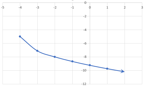
For the function \(f(x) = -3\sqrt{0.5x+2}-5\):
- Identify the parent function
- Identify the transformations that were applied
- Determine the domain and range
- Sketch the transformed function
i. We can identify the parent function as \(f(x) = \sqrt{x}\).
ii. After shifting some of the values in the transformed equation, we can represent it as:
We can now determine the transformations more easily:
- \(a = -3\); vertical stretch by a factor of 3 and reflection in \(x\)-axis
- \(k = 0.5\); horizontal stretch by a factor of \(2\)
- \(d = -4\); shifted left \(4\) units
- \(c = -5\); shifted downward \(5\) units
iii. We can identify the domain and range as such:
- Domain: \(\{x\in\mathbb{R} | x \ge 4\}\)
- Range: \(\{y\in\mathbb{R} | y \ge 5\}\)
iv. We can sketch our transformed graph as such:
Shortcuts for Transforming Functions
Since we've had some experience transforming functions, we can use the following steps to make the process more convenient for sketching the transformed functions:
- Factor out \(k\) to see \(d\)
- Fill out the 3 tables below
- Plot the final table
Example
Write the equation for the following transformed function. Sketch using the shortcut:
\(f(x) = |x|\) reflected in the \(x\)-axis, horizontal compression by a factor of \(2\), shift up \(5\) units.
Before writing out our equation, we can identify the transformations:
- \(a = -1\)
- \(k = 2\)
- \(c = 5\)
Now, we can write the equation of the transformed function:
Finally, we can use our shortcut tables to help draw our graph:
| x | -3 | -2 | -1 | 0 | 1 | 2 | 3 |
|---|---|---|---|---|---|---|---|
| f(x) (Parent) | 3 | 2 | 1 | 0 | 1 | 2 | 3 |
| x ÷ 2 | -1.5 | -1 | -0.5 | 0 | 0.5 | 1 | 1.5 |
|---|---|---|---|---|---|---|---|
| f(x) . (-1) | -3 | -2 | -1 | 0 | -1 | -2 | -3 |
| x | -1.5 | -1 | -0.5 | 0 | 0.5 | 1 | 1.5 |
|---|---|---|---|---|---|---|---|
| f(x) + 5 | 2 | 3 | 4 | 5 | 4 | 3 | 2 |
Now, we can draw our transformed graph as such:

\(g(x) = x^3\) reflected in the \(y\)-axis, horizontal stretch by a factor of \(3\), vertical compression by a factor of \(2\), shift left \(4\) units.
Before writing out our equation, we can identify the transformations:
- \(a = 1/2\)
- \(k = -1/3\)
- \(d = -4\)
Now, we can write the equation of the transformed function:
Finally, we can use our shortcut tables to help draw our graph:
| x | -3 | -2 | -1 | 0 | 1 | 2 | 3 |
|---|---|---|---|---|---|---|---|
| g(x) (Parent) | -27 | -8 | -1 | 0 | 1 | 8 | 27 |
| x ÷ (-1/3) | 9 | 6 | 3 | 0 | -3 | -6 | -9 |
|---|---|---|---|---|---|---|---|
| y . 1/2 | -13.5 | -4 | -0.5 | 0 | 0.5 | 4 | 13.5 |
| x - 4 | 5 | 2 | -1 | -4 | -7 | -10 | -13 |
|---|---|---|---|---|---|---|---|
| g(x) | -13.5 | -4 | -0.5 | 0 | 0.5 | 4 | 13.5 |
Now, we can draw our transformed graph as such:
![Graph of transformed cubic function, g(x)=1/2[-1/3(x+4)]³.](CubicFunction.PNG)