Scalar Multiples
Scalar Multiples are the products of a vector by a scalar value. During this process, the magnitude is multiplied by the scalar and the vectors are parallel to each other.
A scalar multiple can either stretch or compress the vector depending on its value. The direction remains unchanged if the scalar is positive and becomes opposite if the scalar is negative.
Example
Consider vector \(\vec{v}\) with magnitude \(|\vec{v}| = 30[\text{m/s}]\) and a quadrant bearing of \(N60^{\circ}W\).
Use the following scalar vectors to determine the respective resultant vectors:
- \(2\vec{v}\)
- \(0.5\vec{v}\)
- \(-3.5\vec{v}\)
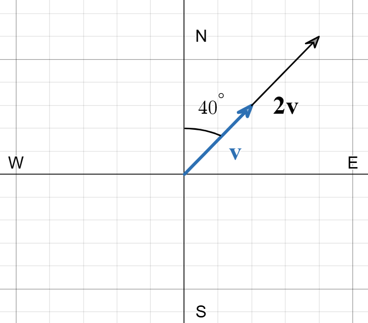
i. In order to determine the resultant vector, we can multiply the magnitude of the original vector by a factor of \(2\):
\(2\vec{v} = 2(30[\text{m/s}])\)
\(2\vec{v} = 60[\text{m/s}]\)
Additionally, since the scalar vector is positive, the quadrant bearing stays the same.
Therefore, we can determine that \(2\vec{v}\) is \(\boldsymbol{60[\textbf{m/s}]}\) with a quadrant bearing of \(\boldsymbol{N60^{\circ}W}\).
ii. In order to determine the resultant vector, we can multiply the magnitude of the original vector by a factor of \(0.5\):
\(0.5\vec{v} = 0.5(30[\text{m/s}])\)
\(0.5\vec{v} = 15[\text{m/s}]\)
Additionally, since the scalar vector is positive, the quadrant bearing stays the same.
Therefore, we can determine that \(0.5\vec{v}\) is \(\boldsymbol{15[\textbf{m/s}]}\) with a quadrant bearing of \(\boldsymbol{N60^{\circ}W}\).
iii. In order to determine the resultant vector, we can first multiply the magnitude of the original vector by a factor of \(3.5\):
\(3.5\vec{v} = 3.5(30[\text{m/s}])\)
\(3.5\vec{v} = 105[\text{m/s}]\)
Additionally, since the scalar vector is negative, the quadrant bearing is reversed.
Therefore, we can determine that \(-3.5\vec{v}\) is \(\boldsymbol{105[\textbf{m/s}]}\) with a quadrant bearing of \(\boldsymbol{S60^{\circ}E}\).
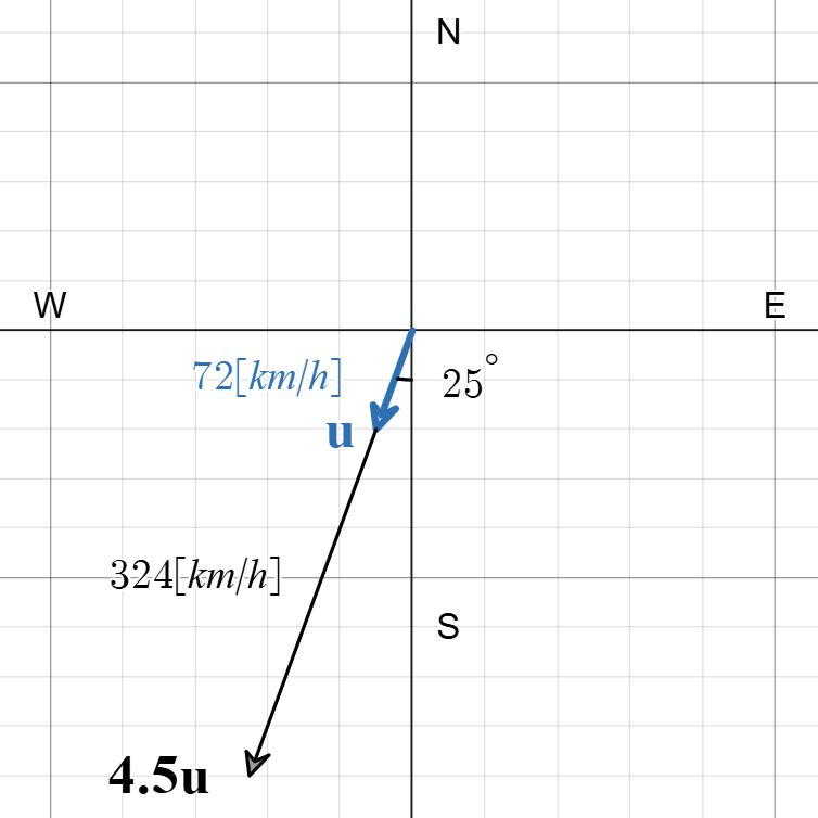
\(4.5\vec{u}\)
In order to determine the resultant vector, we can multiply the magnitude of the original vector by a factor of \(4.5\):
\(4.5\vec{u} = 4.5(72[\text{km/h}])\)
\(4.5\vec{u} = 324[\text{km/h}]\)
Additionally, since the scalar vector is positive, the quadrant bearing stays the same.
Therefore, we can determine that \(4.5\vec{u}\) is \(324[\text{km/h}]\) with a quadrant bearing of \(S25^{\circ}W\).
In order to draw the vector, we will need to draw an arrow \(4.5\) times as long as \(\vec{u}\), in the same direction as \(\vec{u}\):
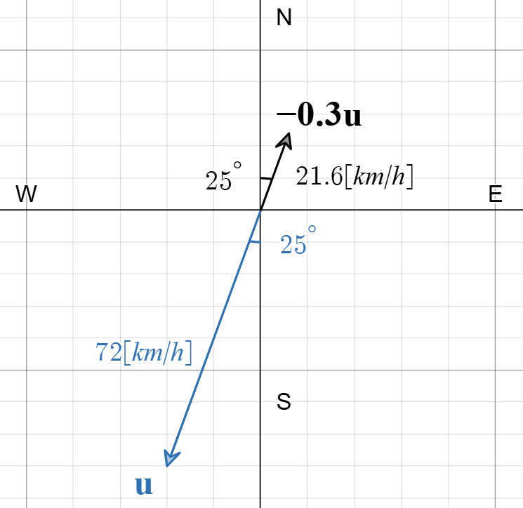
\(-0.3\vec{u}\)
In order to determine the resultant vector, we can multiply the magnitude of the original vector by a factor of \(0.3\):
\(-0.3\vec{u} = 0.3(72[\text{km/h}])\)
\(-0.3\vec{u} = 21.6[\text{km/h}]\)
Additionally, since the scalar vector is negative, the quadrant bearing is reversed.
Therefore, we can determine that \(-0.3\vec{u}\) is \(21.6[\text{km/h}]\) with a quadrant bearing of \(N25^{\circ}E\).
In order to draw the vector, we will need to draw an arrow \(0.3\) times as long as \(\vec{u}\), in the opposite direction as \(\vec{u}\):
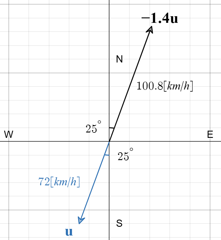
\(-1.4\vec{u}\)
In order to determine the resultant vector, we can multiply the magnitude of the original vector by a factor of \(1.4\):
\(-1.4\vec{u} = 1.4(72[\text{km/h}])\)
\(-1.4\vec{u} = 100.8[\text{km/h}]\)
Additionally, since the scalar vector is negative, the quadrant bearing is reversed.
Therefore, we can determine that \(-1.4\vec{u}\) is \(100.8[\text{km/h}]\) with a quadrant bearing of \(N25^{\circ}E\).
In order to draw the vector, we will need to draw an arrow \(1.4\) times as long as \(\vec{u}\), in the opposite direction as \(\vec{u}\):
Vector Properties of Scalar Multiplications
The following outlines the different rules for scalar multiplication:
- Distributive Property: For any scalar, \(k \in \mathbb{R}\), and any vectors \(\vec{u}\) and \(\vec{v}\), \(k(\vec{u} + \vec{v}) = k\vec{u} + k\vec{v}\)
- Associative Property: For any scalars \(a\) and \(b \in \mathbb{R}\) and any vector \(\vec{v}\), \((ab)\vec{v} = a(b\vec{v})\)
- Identity Property: For any vector, \(\vec{v}\), \(1\vec{v} = \vec{v}\)
Example
Simplify each of the following expressions algebraically:
- \(\vec{u} + \vec{v} + 3\vec{u}\)
- \(2(\vec{u} - \vec{v})-4\vec{u}+\vec{u}\)
i. First, we can use commutative property to rerrange the terms in the expression:
\(= \vec{u} + 3\vec{u} - \vec{v}\)
Next, we can simplify the expression by collecting like terms:
\(= 4\vec{u} - \vec{v}\)
Therefore, we can determine the simplified expression is \(\boldsymbol{4\vec{u} - \vec{v}}\).
ii. First, we can use distributive property to expand the expression:
\(= 2(\vec{u}) - 2(\vec{v})-4\vec{u}+\vec{u}\)
\(= 2\vec{u} - 2\vec{v}-4\vec{u}+\vec{u}\)
Next, we can use commutative property to rerrange the terms in the expression:
\(= 2\vec{u} + \vec{u} - 2\vec{v}-4\vec{u}\)
Then, we can simplify the expression by collecting like terms:
\(= 3\vec{u} - 6\vec{v}\)
Therefore, we can determine the simplified expression is \(\boldsymbol{3\vec{u} - 6\vec{v}}\).
\(-(2\vec{v} - 6\vec{u}) + 3(3\vec{u} - \vec{v})\)
First, we can use distributive property to expand the expression:
\(= -(2\vec{v}) -(-6\vec{u}) + 3(3\vec{u}) - 3(\vec{v})\)
\(= -2\vec{v} + 6\vec{u} + 9\vec{u} - 3\vec{v}\)
Next, we can use commutative property to rerrange the terms in the expression:
\(= -2\vec{v} - 3\vec{v} + 6\vec{u} + 9\vec{u}\)
Then, we can simplify the expression by collecting like terms:
\(= -5\vec{v} + 15\vec{u}\)
Therefore, we can determine the simplified expression is \(\boldsymbol{-5\vec{v} + 15\vec{u}}\).
\(5\vec{v} + 2(\vec{u}+\vec{v}) - 8\vec{u} - 4(\vec{u}-3\vec{v})\)
First, we can use distributive property to expand the expression:
\(= 5\vec{v} + 2(\vec{u}) + 2(\vec{v}) - 8\vec{u} - 4(\vec{u}) -4(-3\vec{v})\)
\(= 5\vec{v} + 2\vec{u} + 2\vec{v} - 8\vec{u} - 4\vec{u} + 12\vec{v}\)
Next, we can use commutative property to rerrange the terms in the expression:
\(= 5\vec{v} + 2\vec{v} + 12\vec{v} + 2\vec{u} - 8\vec{u} - 4\vec{u}\)
Then, we can simplify the expression by collecting like terms:
\(= 19\vec{v} - 10\vec{u}\)
Therefore, we can determine the simplified expression is \(\boldsymbol{19\vec{v} - 10\vec{u}}\).