Linear Regression
Linear Regression is a mathematical function for determining the relationship between a dependent variable and an independent variable. When the two variables have a linear correlation, you can develop a simple mathematical model of the relationship between the two variables by finding a line of best fit, which is a line that displays the general trend of a set of data points on a graph.
But, how do we know if the line of best fit is a good estimate of the trend? Well, we could eyeball it and look at the graph, but there is an analytical approach to this using the residual values of the graph and least-squares fit.
Residuals
A Residual value refers to the vertical distance between each of the data points and the line of best fit. The regression matters because it indicates how well our line of best fit reflects the data.
The formula for Residuals is:
- \(\text{Actual}\; Y\) is the data point on the grap
- \(\text{Predicted}\; Y\) is the point in which the residual line and the regression line intersect each other
The quantity of the regression value tells us how well the line of best fit reflects the data.
- If residuals are small, the model is making accurate predictions
- If residuals are large, the model is not fitting the data well
The sign of the regression value also matters in this context:
- If it's a positive residual, The actual value is higher than the predicted value (the model underestimates)
- If it's a negative residual, The actual value is lower than the predicted value (the model overestimates)
- If the Residual is equal to 0, The prediction is exactly correct for that value

It's important to watch out for outliers in your graph. These are values that vary drastically from the line of best fit. These points might negatively influence the line of best fit. In order to prevent this, remove the outlier and recalculate the regression line.
In order to determine the residual value, we can use the following formula:
Using the above formula, we can compute the following:
\(\text{Residual} = 3 - 1\)
\(\text{Residual} = 2\)
Therefore, we can determine the residual for this point is 2.
Least-Squares Fit
The least-squares fit is a mathematical method used to find the best-fit line for a set of data points. Ideally, we want the sum of all residuals to be zero and the sum of the squares of the residuals should be as small as possible.
The sum of squared residuals \((SSR\)) can be be calculated as such:
- \(y_{\text{actual}}\) is the observed value from the dataset.
- \(y_{\text{predicted}}\) is the predicted value from the regression line.
- \((y_{\text{actual}} - y_{\text{predicted}})\) is the residual for each data point.
- Summation Symbol (\(\sum\)) means we add up all of the squared residuals in the dataset.
Although the algebra looks daunting, the equation of this line can be determined using:
Where \(\bar{x}\) is the mean of \(x\) and \(\bar{y} \) is the mean of \(y\).
Note: You might also see this referenced as \(y = ax + b \). It's the same equation, with \(a\) as the slope.
Interpolating and Extrapolating
Using the line of best fit, You can then use the equation for this line to make predictions by interpolating and extrapolating the data.
Interpolating means predicting values that lie within the domain/range. These values are within the data that we have collected. In simple terms, we are predicting values anywhere in between the first data point and the last data point of our Scatter Plot.
Extrapolating means predicting values that lie outside the domain or range. These values are outside the data that we've collected. Usually when doing extrapolation, we present our predictions with a disclaimer saying “If the model continues this way, then…”. We do this, as we have no trends to aid us in our predictions, thus we don’t know for sure what will happen.
A cyclist modelled the relationship between the time he cycles, and the amount of distance he covers, in Miles, in the following table.
- What are the Independant and Dependant Variables?
- How far does he travel in 12 minutes?
| Time He Cycles (Minutes) | Distance He Covers (Miles) |
|---|---|
| 10 | 4.0 |
| 20 | 5.9 |
| 30 | 7.0 |
| 40 | 8.5 |
| 50 | 9.8 |
i. The Independant variable (or \(x\)-value) is how much time he cycles in minutes, and the Dependant variable (or \(y\)-value) is how much distance he covers in miles.
ii. First, we can sketch a graph to more easily determine a formula to represent the cyclist's distance:
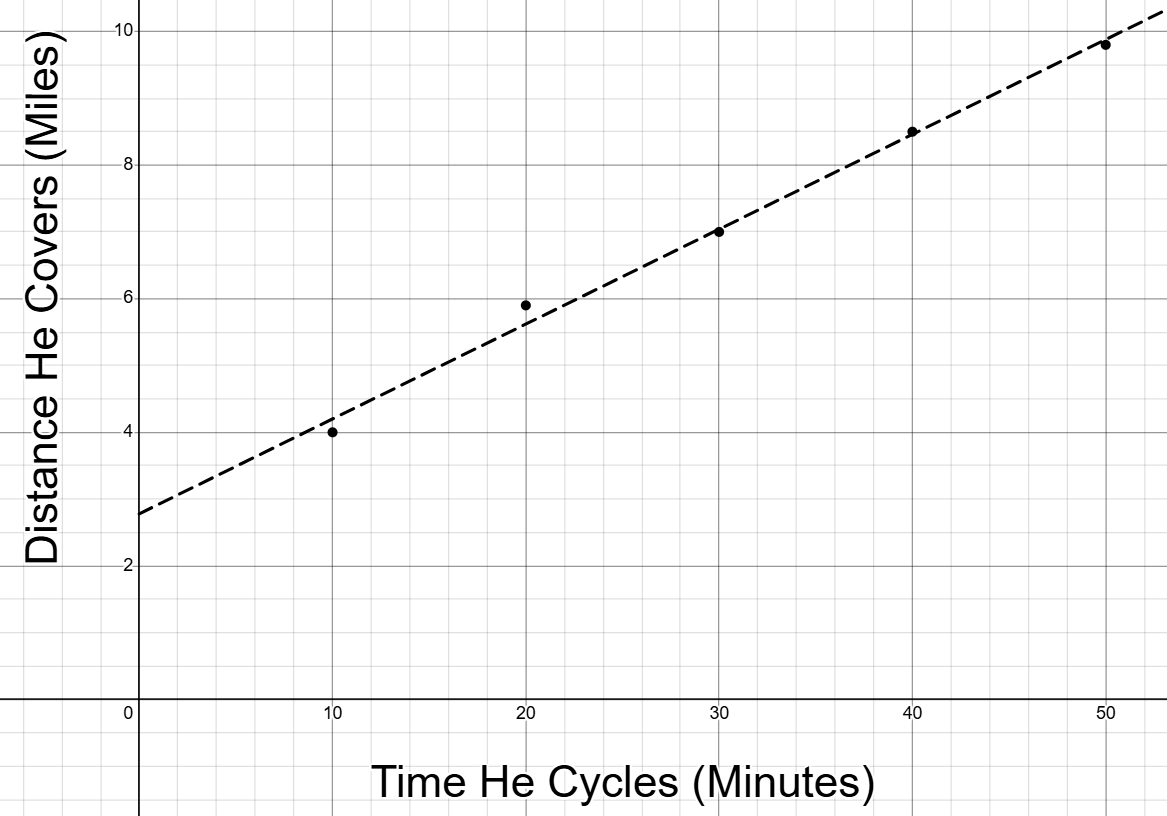
Based on this graph, we can represent the distance algebraically as such:
In order to determine the cyclist's distance after \(12\) minutes, we can substitute this value into the equation:
\(y = 0.142x + 2.78\)
\(y = 0.142 (12) + 2.78\)
\(y = 4.484\)
Therefore, we can determine the cyclist's distance after \(12\) minutes is approximately 4.5 miles.