Measures Of Spread
Measures of spread describe how data points in a dataset vary. They help understand how much the data is scattered or clustered around the center.
Standard Deviation and Variance
Variance measures how far each number in the dataset is from the mean. It is found by averaging the squared differences from the mean.
The formula for population variance is:
The formula for sample variance is:
Standard deviation is the square root of variance. It shows how spread out the numbers are in the same units as the data.
The formula for population standard deviation is:
The formula for sample standard deviation is:
Outlined below are the key differences between Variance and Standard Deviation:
| Feature | Variance (\(\sigma^2\)) | Standard Deviation (\(\sigma\)) |
|---|---|---|
| Definition | Measures the average squared deviation from the mean | Measures how spread out the data is, but in the same unit as the data |
| Formula | \[ \sigma^2 = \frac{\sum (x - \bar{x})^2}{N} \] | \[ \sigma = \sqrt{\text{variance}} \] |
| Unit | Squared unit of the original data | Same unit as the original data |
| Interpretation | Harder to interpret because of squared units | Easier to understand as it relates directly to data spread |
Example
Determine the Standard Deviation of a group of students with test scores of 50, 60, 70, 80, and 90.
First, we can determine the mean of the test scores:
\(\text{Mean} = \cfrac{50 + 60 + 70 + 80 + 90}{5}\)
\(\text{Mean} = 70 \)
Next, we can determine the variance of the test scores:
\(\sigma^2 = \cfrac{(50-70)^2 + (60-70)^2 + (70-70)^2 + (80-70)^2 + (90-70)^2}{5}\)
\(\sigma^2 = \cfrac{(-20)^2 + (-10)^2 + (0)^2 + (10)^2 + (20)^2}{5}\)
\(\sigma^2 = \cfrac{400 + 100 + 0 + 100 + 400}{5}\)
\(\sigma^2 = \cfrac{1000}{5}\)
\(\sigma^2 = 200\)
Then, we can determine the standard deviation of the test scores:
Standard deviation (\(\sigma\)) is the square root of variance:
\(\sigma = \sqrt{200}\)
\(\sigma \approx 14.14\)
Therefore, we can determine the Standard Deviation of the students' test scores is ~ 14.14.
Box and Whisker Plots
Box plots (or box-and-whisker plots) visually display the spread of data using five key numbers:
- Minimum - smallest value
- First Quartile (Q1) - 25% of data below this point
- Median (Q2) - middle value
- Third Quartile (Q3) - 75% of data below this point
- Maximum - largest value
The following box-and-whisker plot represents a dataset of [1, 3, 5, 7, 9, 11, 13], Q1 = 3, Q2 (median)= 7, and Q3 = 11.
![A Box and Whisker Plot representing a dataset of [1, 3, 5, 7, 9, 11, 13] with a Q1 of 3, median of 7, and Q3 of 11.](BOXPLOT.png)
Quartiles and Interquartile Range (IQR)
Quartiles divide the data into four equal parts. The interquartile range (IQR) is the difference between Q3 and Q1. It shows the range of the middle 50% of the data, reducing the impact of extreme values.
The Interquartile Range (IQR) can be determined algebraically as such:
Where:
- \(Q_1\) = First quartile (25th percentile)
- \(Q_3\) = Third quartile (75th percentile)
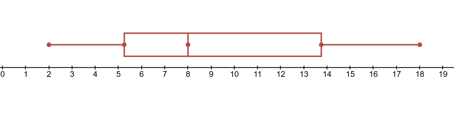
The following Box and Whisker Plot represents a \(Q_1\) of \(5.5\), a \(Q_3\) of \(13.5\), and IQR of \(8\).
 Example
Determine the Interquartile Range if Q1 = 5 and Q3 = 15.
In order to determine the Interquartile Range, we can substitute the pertinent values into the corresponding formula and solve:
\(\text{IQR} = Q_3 - Q_1\)
\(\text{IQR} = 15 - 5\)
\(\text{IQR} = 10\)
Therefore, we can determine that the Interquartile Range is 10.
Percentiles and Percentile Rank
A Percentile indicates what percentage of the data falls below a particular value. For example, the 90th percentile means the value is greater than 90% of the data.
The Percentile Rank is the position of a value relative to the rest of the dataset.
We can determine the location of the \(pth\) percentile algebraically as such:
Where:
- \(L_p\) refers to the position of the percentile
- \(p\) refers to the \(pth\) percentile
- \(n\) refers to the number of total data points
We can determine the \(pth\) percentile algebraically as such:
Where:
- \(Y_p\) refers to the percentile value
- \(f_p\) refers to the fractional component of \(L_p\)
- \(i_p\) refers to the integer component of \(L_p\)
- \(x_{i_{p}}\) refers to element \(L_p\) is closest to
- \(x_{i_{p + 1}}\) refers to element that comes after \(x_{i_{p}}\)
Z-Scores
The Z-Score shows how many standard deviations a value is from the mean. A positive Z-score means the value is above the mean, while a negative Z-score means it is below the mean.
Here is the formula for a Z-score:
Where:
- \(Z\) is the Z-score
- \(X\) is the data point
- \(\mu\) is the population mean
- \(\sigma\) is the population standard deviation
Example
Determine the \(Z\)-Score of a student if their test score was 75, the mean is 70, and the Standard Deviation is 5.
In order to determine the student's \(Z\)-Score, we can substitute the pertinent values into the corresponding formula and solve:
\(Z = \cfrac{X - \mu}{\sigma}\)
\(Z = \cfrac{75 - 70}{5}\)
\(Z = 1\)
Therfore, we can determine the student's \(Z\)-Score is 1.
The difference between the two plots is a regular box and whisker plot includes all data points in its whiskers, whereas a modified box-and-whisker plot separates outliers to make the spread of typical data clearer.
Since the values are already arranged in ascending order, we don't need to rearrange anything further.
Next, we can find the median of the data set (or Q2). Since this dataset contains 11 values, the median is represented by the 6th value. In this case, it is 24.
Then, we can find the median of the lower quartile (or Q1). The lower half of the dataset is [12, 15, 18, 21, 22]. The median of this set is 18. So, Q1 = 18.
After, we can find the median of the upper quartile (or Q3). The upper half of the data set is [30, 33, 35, 40, 50]. The median of this set is 35. So, Q3 = 35.
Finally, we can determine the IQR by susbstituting the values into corresponding formula and solving:
\(\text{IQR} = Q3 - Q1\)
\(\text{IQR} = 35 - 18\)
\(\text{IQR} = 17\)
Therefore, we can determine the IQR is 17.
In order to determine the student's \(Z\)-Score, we can substitute the pertinent values into the corresponding formula and solve:
\(Z = \cfrac{X - \mu}{\sigma}\)
\(Z = \cfrac{82 - 70}{8}\)
\(Z = 1.5\)
Therefore, we can determine the \(Z\)-score is 1.5, indicating the student scored 1.5 Standard Deviations above the mean.
Since the values are already arranged in ascending order, we don't need to rearrange anything further.
Next, we can use the Rank formula:
We can substitute the percentile value \(P = 40\) and number of data points (\(N = 10\)) into the formula to determine the Rank:
\(L_p = \cfrac{40}{100} \times (10 + 1)\)
\(L_p = 0.4 \times 11\)
\(L_p = 4.4\)
Since 4.4 is between the 4th and 5th data points , we can calculate the 40th percentile value as such:
\(Y_p = x_{i_{p}} + f_p \times (x_{i_{p+1}} - x_{i_{p}})\)
\(Y_p = 75 + 0.4 \times (80 - 75)\)
\(Y_p = 75 + 2\)
\(Y_p = 77\)
Therefore, we can determine the 40th percentile is 77.