Trigonometry - Word Problems
Outlined below are some steps, tips, and strategies that should be helpful for solving word problems the involve trigonometric functions:
- Take domain constraints into account when determining the solutions of a trigonometric function
- Use the amplitude and vertical axis in order to determine the max and min points of a function or vice versa
- Use the k value (if it exists) to determine the period of a function. This will help you determine the interval between different extrema
- In order to make a unit conversion, identify the unit of your current value and multiply it by the appropriate ratio:
- If you want to convert revolutions to radians, multiply the value by \(2π\;[\text{rads}]/1\; [\text{rev}]\)
- If you want to convert radians to revolutions, multiply the value by \(1\;[\text{rev}]/2π \;[\text{revs}]\)
- The above also applies to time-related units:
- To convert seconds to minutes, multiply the value by \(1\;[\text{min}]⁄60\;[\text{sec}]\)
- To convert minutes to seconds, multiply the value \(60\;[\text{sec}]⁄1\;[\text{min}]\)
- Look at what trigonometric ratio the expression uses to identify where the starting point is located or how the function appears graphically
- Make sure to include units in the final answers!
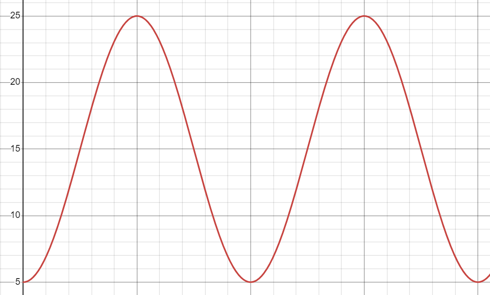
A mass on a spring is pulled toward the floor and released, causing it to move up and down. Its height, in centimeters, above the floor after \(t\) seconds is given by the function \(h(t) = 10\sin(2\pi t + 1.5\pi) + 15, 0 \leq t \leq 2\).
- Sketch the graph of height vs. time
- What does the rate of change of this function represent?
- Predict for which \(2\) points the instantaneous rate of change is \(0\)
- Predict for which \(2\) intervals the average rate of change is positive on one and negative on the other but contains the same values regardless.
i. First, we need to determine the period, axis, max and min points in order to accurately draw the graph.
We can identify half the period's length by dividing \(2\pi\) by \(k\), \(2\pi\):
\(p = \cfrac{2\pi}{k}\)
\(p = \cfrac{2\pi}{2\pi}\)
\(p = 1\)
Next, the axis, \(c\), is already to us in the function (\(15\)).
Then, we can find the max and min points by respectively adding and subtracting the amplitude, \(10\) to the axis.
We can find the max point as such:
\(\text{max} = \text{axis} + \text{amplitude}\)
\(\text{max} = 15 + 10\)
\(\text{max} = 25\;[\text{cm}]\)
We can find the min point as such:
\(\text{min} = \text{axis} - \text{amplitude}\)
\(\text{min} = 15 - 10\)
\(\text{min} = 5\;[\text{cm}]\)
Using this information, we can create a table of values:
| Time (s) | \(0\) | \(0.25\) | \(0.5\) | \(0.75\) | \(1\) |
|---|---|---|---|---|---|
| Height Above Ground (cm) | \(5\) | \(15\) | \(25\) | \(15\) | \(5\) |
We can now draw our graph:
ii. The Rate of Change can be algebraically represented as such:
The rate of change represents the spring's change in height above the floor in relation to the change in time (or its linear speed).
iii. The instantaneous rate of change is \(0\) when \(m_{\tan} = 0\). This can be found at the turning points when there is no slope, which in this instance are found at \(\boldsymbol{x = 0, 5}\).
iv. Two intervals where the intervals share the same values but different rates of change are \(\boldsymbol{x \in [1.25, 1.5]}\) and \(\boldsymbol{x \in [1.5, 1.75]}\).
The first interval contains a positive \(m_{\sec}\) while the second interval contains a negative \(m_{\sec}\).
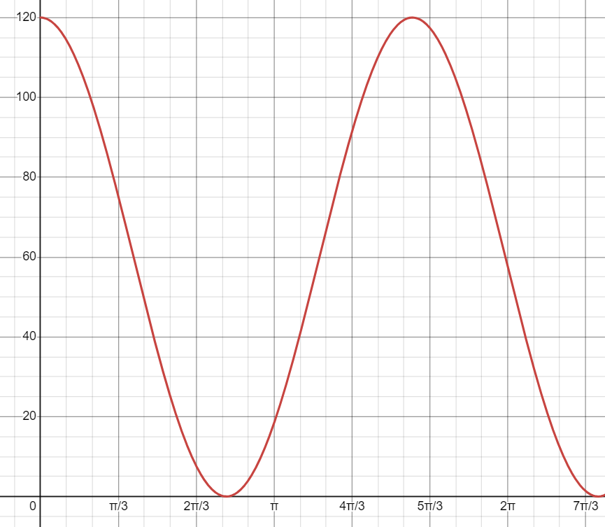
Commercial bottling machines often use a circular drum as part of a mechanism to install tops on bottles. One such machine has a diameter of \(120\;[\text{cm}]\) and makes a complete turn every \(5\;[\text{s}]\). A sensor at the left side of the drum monitors its movement. Take the sensor position as zero.
- Sketch the graph of the horizontal position of a point on the drum, \(h\). In centimeters, as a function of time, \(t\), in seconds.
- What is the equation that models this?
- What is the position of a point on the drum in \(1\) minute after the machine has started?
- At what time in the first \(10\) second interval is a point on the drum \(50\;[\text{cm}]\) away horizontally from the sensor?
i. First, we need to determine the period and axis in order to accurately draw the graph.
We can identify half the period's length by subtracting the time at the min point, \(2.5\), by the time at the max point, \(0\). We can then multiply that value by \(2\) to get the full period length:
\(\cfrac{1}{2}\text{period} = 2.5 - 0\)
\(\text{period} = (2.5)(2)\)
\(\text{period} = 5\;[\text{sec}]\)
Next, we need to determine the axis. We can do so by finding the average of the max and min points:
\(\text{axis} = \cfrac{120 + 0}{2}\)
\(\text{axis} = \cfrac{120}{2}\)
\(\text{axis} = 60\;[\text{cm}]\)
Using this information, we can create a table of values:
| Time (s) | \(0\) | \(1.25\) | \(2.5\) | \(3.75\) | \(5\) |
|---|---|---|---|---|---|
| Horizontal Position (cm) | \(120\) | \(60\) | \(0\) | \(60\) | \(120\) |
We can now draw our graph:
ii. As a reference, our formula can be represented as a cosine function in the form \(h(t) = |a|\cos[k(t - d)] + c\). This is because \(x = 0\) represents the function's max point, like that of a cosine function.
First, we can find the amplitude by subtracting the maximum by the minumum and dividing the result by \(2\):
\(\text{amplitude} = \cfrac{120 - 0}{2}\)
\(\text{amplitude} = \cfrac{120}{2}\)
\(\text{amplitude} = 60\;[\text{cm}]\)
Next, we can find \(k\) through dividing \(2\pi\) by the period length, \(5\):
\(k = \cfrac{2\pi}{5}\)
Then, we can determine \(d\) by finding the first \(t\)-value that corresponds to a peak. By looking at our graph, we can determine that this point lies at \(0\).
We have already determined the axis (or \(c\)) in Part i. As a result, we can put our formula together:
\(\boldsymbol{h(t) = 60\cos\left[\cfrac{2\pi}{5}\left(t - 0\right)\right] + 60}\)
iii. In order to determine the position on the drum \(1\) minute after the machine has started, we can set \(t = 60\) and solve the equation:
\(h(60) = 60\cos\left[\cfrac{2\pi}{5}\left(60\right)\right] + 60\)
\(h(60) = 60\cos(75.39822369) + 60\)
\(h(60) = 60(1) + 60\)
\(h(60) = 60 + 60\)
\(h(60) = 120\;[\text{cm}]\)
Therefore, we can determine the position on the drum after \(1\) minute is \(\boldsymbol{120\; [\textbf{cm}]}\).
iv. In order to determine the times that the spring was \(50\;[\text{cm}]\) horizontally from the sensor, we can first set the function equal to \(50\). We can also represent \(\cfrac{2\pi}{5}t\) as \(\theta\):
We can then simplify the expression as such:
\(\cfrac{-10}{60} = \cfrac{60\cos(\theta)}{60}\)
\(-\cfrac{1}{6} = \cos(\theta)\)
Next, we can find the inverse of \(\cos\) to calcualte \(\theta\):
\(\theta_1 = \cos\left(-\cfrac{1}{6}\right)^{-1}\)
\(\theta_1 = 1.738 \; [\text{rads}]\)
We can determine that this ratio lies in Quadrants 2 and 3 since those are the quadrants where the cosine function is negative.
Since the second solution is located in Quadrant \(3\), we can determine its value by subtracting the first solution from \(2\pi\):
\(\theta_2 = 2\pi\;[\text{rads}] - 1.74\; [\text{rads}]\)
\(\theta_2 = 4.545 \; [\text{rads}]\)
In order to determine \(t\), we can now set \(\theta\), \(\cfrac{2\pi}{5}t\), equal to the solutions.
We can determine the first solution as such:
\(\cfrac{2\pi}{5}t_1 = 1.738\)
\(t_1 = \left(\cfrac{5}{2\pi}\right)(1.738)\)
\(t_1 = 1.38\;[\text{sec}]\)
We can determine the second solution as such:
\(\cfrac{2\pi}{5}t_2 = 4.545\)
\(t_2 = \left(\cfrac{5}{2\pi}\right)(4.545)\)
\(t_2 = 3.62\;[\text{sec}]\)
In order to determine other possible solutions for \(t\), we can add \(5\;[\text{sec}]\) to the provided times.
We can determine the third solution as such:
\(t_3 = 1.38 + 5\)
\(t_3 = 6.38\;[\text{sec}]\)
We can determine the fourth solution as such:
\(t_4 = 3.62 + 5\)
\(t_4 = 8.62\;[\text{sec}]\)
Therefore, we can determine the times within the first \(10\) seconds that a point on the drum is \(50\;[\text{cm}]\) away from the sensor are \(\boldsymbol{1.38\;[\text{sec}], 3.62\;[\text{sec}], 6.38\;[\text{sec}], 8.62 \; [\text{sec}]}\).
First, we can convert the plane's linear velocity from km/h to m/sec:
\(v \approx 180.56 \left[\cfrac{\text{m}}{\text{sec}}\right]\)
Next, we can calculate the circumference of the circle the plane is flying. This circle represents the distance the plane travels in one rotation:
\(C = 2\pi r\)
\(C = 2\pi \times 8\;[\text{m}]\)
\(C = 16\pi [\text{m}]\)
Then, we can determine the Number of rotations the plane makes per second by dividing the linear velocity, \(v\) by the circumference, \(C\):
\(\text{# of rotations/second} = \cfrac{180.56 \left[\cfrac{\text{m}}{\text{sec}}\right]}{16\pi [\text{m}]}\)
\(\text{# of rotations/second} = \cfrac{180.56 {\cancel{[\text{m}]}}}{[\text{sec}]} \times \cfrac{1\;[\text{rotations}]}{16\pi \cancel{[\text{m}]}}\)
\(\text{# of rotations/second} = \cfrac{180.56 \; [\text{rotations}]}{16\pi\;[\text{seconds}]}\)
After, we can simplify the expression as such:
Therefore, we can determine that the plane makes \(\boldsymbol{\approx 3.6 \left[\cfrac{\textbf{rotations}}{\textbf{sec}}\right]}\).