Polynomials - Transformations
There are various transformations that can be applied to parent functions in order to change their core attributes. A transformed function can be expressed algebraically as:
- \(a\) represents the vertical stretch/compression factor.
- \(k\) represents the horizontal stretch/compression factor
- \(d\) represents the horizontal shift
- \(c\) represents the vertical shift
- \(n\) represents the degree
Vertical Stretch/Compression
The value of \(a\) will determine whether the transformed function will be vertically stretched or compressed:
- If \(a > 1\), the function will be vertically stretched
- If \(0 < a < 1\), the function will be vertically compressed
- If \(a < 0\), the function will either be vertically stretched or compressed with a reflection in the x-axis
Horizontal Stretch/Compression
The value of \(k\) will determine whether the transformed function will be horizontally stretched or compressed:
- If \(0 < k < 1\), the function will be horizontally stretched by a factor of 1/k
- If \(k > 1\), the function will be horizontally compressed by a factor of 1/k
- If \(k < 0\), the function will either be horizontally stretched or compressed with a reflection in the y-axis
Horizontal Shift
The value of \(d\) will determine whether the transformed function will be shifted left or right:
- If \(d > 0\), the function will be shifted right
- If \(d < 0\), the function will be shifted left
Vertical Shift
The value of \(c\) will determine whether the transformed function will be shifted upward or downward:
- If \(c > 0\), the function will be shifted upward
- If \(c < 0\), the function will be shifted downward
Example
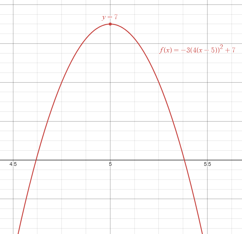
For the function \(f(x) = -3(4x-20)^2+7\):
- Identify the parent function
- Identify the transformations that were applied
- Determine the domain and range
- Sketch the transformed function
i. We can identify the parent function as \(\boldsymbol{f(x) = x^2}\).
ii. After shifting some of the values in the transformed equation, we can represent it as:
We can now determine the transformations more easily:
- \(\boldsymbol{a = -3}\); vertical stretch by a factor of \(3\) and reflection in the \(x\)-axis
- \(\boldsymbol{k = 4}\); horizontal compression by a factor of \(4\)
- \(\boldsymbol{d = 5}\); shifted right by \(5\) units
- \(\boldsymbol{c = 2}\); shifted upwards \(7\) units
iii. We can identify the domain and range as such:
- Domain: \(\boldsymbol{\{x\in\mathbb{R}\}}\)
- Range: \(\boldsymbol{\{y\in\mathbb{R} | y \leq 7\}}\)
iv. We can draw our transformed graph as such:
For the function \(g(x) = 2(-x-1)^3-6\):
- Identify the parent function
- Identify the transformations that were applied
- Identify the domain and range
- Sketch the transformed function
i. We can identify the parent function as \(\boldsymbol{g(x) = x^3}\).
ii. After shifting some of the values in the transformed equation, we can represent it as:
We can now determine the transformations more easily:
- \(\boldsymbol{a = 2}\); vertical stretch by a factor of \(2\)
- \(\boldsymbol{k = -1}\); reflection in the \(y\)-axis
- \(\boldsymbol{d = -1}\); shifted left by \(1\) unit
- \(\boldsymbol{c = -6}\); shifted downward \(6\) units
We can identify the domain and range as such:
- Domain: \(\boldsymbol{\{x\in\mathbb{R}\}}\)
- Range: \(\boldsymbol{\{y\in\mathbb{R}\}}\)
iv. We can draw our transformed graph as such:
![Graph of transformed Cubic Function expressed as g(x)=1/2[-(x+1)]³-6.](Transformations2.PNG)
Shortcuts for Transforming Functions
Since we've had some experience transforming functions, we can use the following steps to make the process more convenient for sketching the transformed functions:
- Factor out \(k\) to see \(d\)
- Fill out the 3 tables below
- Plot the final table
Example
Write the equation for the following transformed function. Sketch using the shortcut:
\(y = x^5\) reflected in the \(y\)-axis, horizontal stretch by \(2\), horizontal shift up by \(9\) units.
Before writing out our equation, we can determine the transformations:
- \(k = -1/2\)
- \(c = 9\)
Now, we can write the equation of the transformed function:
Finally, we can use our shortcut tables to help draw our graph:
| x | -3 | -2 | -1 | 0 | 1 | 2 | 3 |
|---|---|---|---|---|---|---|---|
| y (Parent) | 243 | 32 | 1 | 0 | -1 | -32 | -243 |
| x ÷ -1/2 | 6 | 4 | 2 | 0 | -2 | -4 | -6 |
|---|---|---|---|---|---|---|---|
| y | 243 | 32 | 1 | 0 | -1 | -32 | -243 |
| x | 6 | 4 | 2 | 0 | -2 | -4 | -6 |
|---|---|---|---|---|---|---|---|
| y + 3 | 246 | 35 | 4 | 3 | 2 | -29 | -240 |
Now, we can draw our transformed graph as such:
![Graph of transformed quintic function expressed as y=[1/2(x)]⁵+3.](Transformations3.PNG)
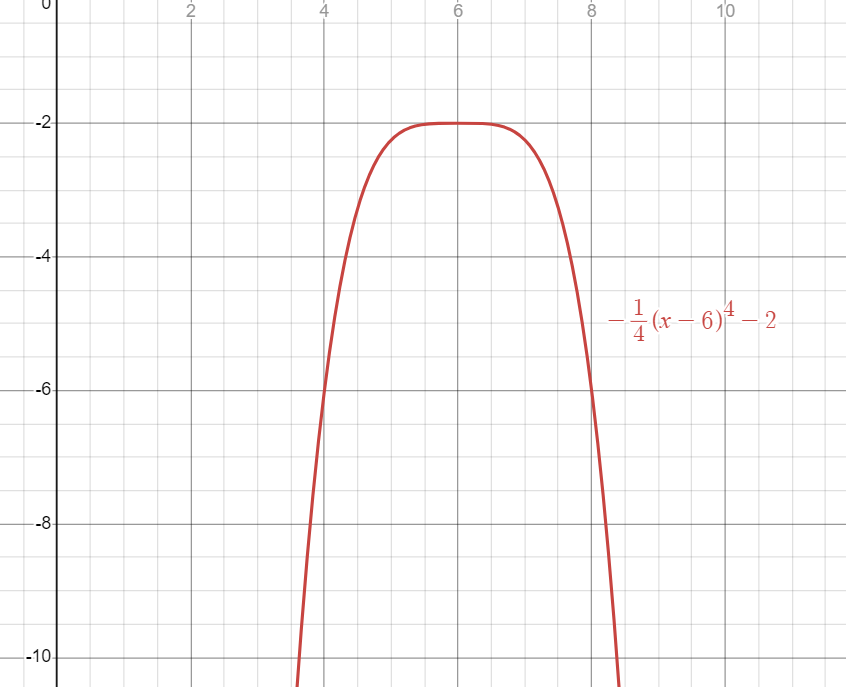
\(i(x) = x^4\) reflected in the \(x\)-axis, vertical compression by \(\cfrac{1}{4}\), shift left \(6\) units, translation \(2\) units downward.
Before writing out our equation, we can determine the transformations:
- \(a = -1/4\)
- \(d = 6\)
- \(c = -2\)
Now, we can write the equation of the transformed function:
Finally, we can use our shortcut tables to help draw our graph:
| x | -3 | -2 | -1 | 0 | 1 | 2 | 3 |
|---|---|---|---|---|---|---|---|
| i(x) (Parent) | 81 | 16 | 1 | 0 | 1 | 16 | 81 |
| x | -3 | -2 | -1 | 0 | 1 | 2 | 3 |
|---|---|---|---|---|---|---|---|
| y . -1/4 | -20.25 | -4 | -0.25 | 0 | -0.25 | -4 | -20.25 |
| x+6 | 3 | 4 | 5 | 6 | 7 | 8 | 9 |
|---|---|---|---|---|---|---|---|
| i(x)-2 | -22.25 | -6 | -2.25 | -2 | -2.25 | -6 | -22.25 |
Now, we can draw our transformed graph as such: